The source code of the hands-on exercises are available at the following link: https://github.com/tomomano/learn-aws-by-coding
🌎Japanese version is available here🌎
1. Introduction
1.1. Purpose and content of this book
This book was prepared as a lecture material for "Special Lectures on Information Physics and Computing", which was offered in the S1/S2 term of the 2021 academic year at the Department of Mathematical Engineering and Information Physics, the University of Tokyo.
The purpose of this book is to explain the basic knowledge and concepts of cloud computing for beginners. It provides hands-on tutorials to use real cloud environment provided by Amazon Web Services (AWS).
We assume that the readers would be students majoring science or engineering at college, or software engineers who are starting to develop cloud applications. We will introduce pracitcal steps to use the cloud for research and web application development. We plan to keep this course as interactive and practical as possible, and for that purpose, less emphasis is placed on the theories and knowledge, and more effort is placed on writing real programs. I hope that this book serves as a stepping stone for readers to use cloud computing in their future research and applications.
The book is divided into three parts:
| Theme | Hands-on | |
|---|---|---|
1st Part (Section 1 to 4) |
Cloud Fundamentals |
|
2nd Part (Section 5 to 9) |
Machine Learning using Cloud |
|
3rd Part (Section 10 to 13) |
Introduction to Serverless Architecture |
|
In the first part, we explain the basic concepts and knowledge of cloud computing. Essential ideas necessary to safely and cleverly use cloud will be covered, including security and networking. In the hands-on session, we will practice setting up a simple virtual server on AWS using AWS API and AWS CDK.
In the second part, we introduce the cocenpts and techniques for running scientific computing (especially machine learning) in the cloud. In parallel, we will learn a modern virtual coumputing environment called Docker. In the first hands-on session, we will run Jupyter Notebook in the AWS cloud and run a simple machine learning program. In the second hands-on, we will create a bot that automatically generates answers to questions using natural language model powered by deep neural network. In the third hands-on, we will show how to launch a cluster with multiple GPU instances and perform massively parallel hyperparameter search for deep learning.
In the third part, we introduce the latest cloud architecture called serverless architecture. This architecture introduces radically different design concept to the cloud than the previous one (often referred to as Serverful), as it allows the processing capacity of the cloud system to be scaled up or down more flexibly depending on the load. In the first hands-on session, we will provide exercises on Lambda, DynamoDB, and S3, which are the main components of the serverless cloud. In addition, we will create a simple yet quite useful social network service (SNS) in the cloud using serverless technology.
These extensive hands-on sessions will provide you with the knowledge and skills to develop your own cloud system on AWS. All of the hands-on programs are designed to be practical, and can be customized for a variety of applications.
1.2. Philosophy of this book
The philosophy of this book can be summed up in one word: "Let’s fly to space in a rocket and look at the earth once!"
What does that mean?
The "Earth" here refers to the whole picture of cloud computing. Needless to say, cloud computing is a very broad and complex concept, and it is the sum of many information technologies, hardware, and algorithms that have been elaborately woven together. Today, many parts of our society, from scientific research to everyday infrastructure, are supported by cloud technology.
The word "rocket" here refers to this lecture. In this lecture, readers will fly into space on a rocket and look at the entire earth (cloud) with their own eyes. In this journey, we do not ask deeply about the detailed machinery of the rocket (i.e. elaborate theories and algorithms). Rather, the purpose of this book is to let you actually touch the cutting edge technologies of cloud computing and realize what kind of views (and applications) are possible from there.
For this reason, this book covers a wide range of topics from the basics to advanced applications of cloud computing. The first part of the book starts with the basics of cloud computing, and the second part takes it to the next level by explaining how to execute machine learning algorithms in the cloud. In the third part, we will explain serverless architecture, a completely new cloud design that has been established in the last few years. Each of these topic is worth more than one book, but this book was written with the ambitious intention of combining them into a single volume and providing a integrative and comprehensive overview.
It may not be an easy ride, but we promise you that if you hang on to this rocket, you will get to see some very exciting sights.

1.3. AWS account
This book provides hands-on tutorials to run and deploy applications on AWS. Readers must have their own AWS account to run the hands-on excercises. A brief description of how to create an AWS account is given in the appendix at the end of the book (Section 14.1), so please refer to it if necessary.
AWS offers free access to some features, and some hands-on excercises can be done for free. Other hands-on sessions (especially those dealing with machine learning) will cost a few dollars. The approximate cost of each hands-on is described at the begining of the excercise, so please be aware of the potential cost.
In addition, when using AWS in lectures at universities and other educational institutions, AWS Educate program is available. This program offers educators various teaching resources, including the AWS credits which students taking the course can use to run applications in the AWS cloud. By using AWS Educate, students can experience AWS without any financial cost. It is also possible for individuals to participate in AWS Educate without going through lectures. AWS Educate provides a variety of learning materials, and I encourage you to take advantage of them.
1.4. Setting up an environment
In this book, we will provide hands-on sessions to deploy a cloud application on AWS. The following computer environment is required to run the programs provided in this book. The installation procedure is described in the appendix at the end of the book (Section 14). Refer to the appendix as necessary and set up an environment in your local computer.
-
UNIX console: A UNIX console is required to execute the commands and access the server via SSH. Mac or Linux users can use the console (also known as a terminal) that comes standard with the OS. For Windows users, we recommend to install Windows Subsystem for Linux (WSL) and set up a virtual Linux environment (see Section 14.5 for more details).
-
Docker: This book explains how to use a virtual computing environment called Docker. For the installation procedure, see Section 14.6.
-
Python: Version 3.6 or later is required. We will also use
venvmodule to run programs. A quick tutorial onvenvmodule is provided in the appendix (Section 14.7). -
Node.js: Version 12.0 or later is required.
-
AWS CLI: WS CLI Version 2 is required. Refer to Section 14.3 for installation and setup procedure.
-
AWS CDK: Version 1.00 or later is required. The tutorials are not compatible with version 2. Refer to Section 14.4 for installation and setup procedure.
-
AWS secret keys: In order to call the AWS API from the command line, an authentication key (secret key) must be set. Refer to Section 14.3 for the setting of the authentication key.
1.5. Docker image for the hands-on exercise
We provide a Docker image with the required programs installed, such as Python, Node.js, and AWS CDK. The source code of the hands-on program has also been included in the image. If you already know how to use Docker, then you can use this image to immediately start the hands-on tutorials without having to install anything else.
Start the the container with the followign command.
$ docker run -it tomomano/labcMore details on this Docker image is given in the appendix (Section 14.8).
1.6. Prerequisite knowledge
The only prerequisite knowledge required to read this book is an elementary level understanding of the computer science taught at the universities (OS, programming, etc.). No further prerequisite knowledge is assumed. There is no need to have any experience using cloud computing. However, the following prior knowledge will help you to understand more smoothly.
-
Basic skills in Python: In this book, we will use Python to write programs. The libraries we will be using are sufficiently abstract that most of the functions make sense just by looking at their names. There is no need to worry if you are not very familiar with Python.
-
Basic skills in Linux command line: When using the cloud, the servers that are launched on the cloud are usually Linux. If you have knowledge of the Linux command line, it will be easier to troubleshoot. If you feel unconfident about using command line, I recommend this book: The Linux Command Line by William Shotts. It is available for free on the web.
1.7. Source code
The source code of the hands-on tutorials is available at the following GitHub repository.
1.8. Notations used in this book
-
Code and shell commands are displayed with
monospace letters -
The shell commands are prefixed with
$symbol to make it clear that they are shell command. The$must be removed when copying and pasting the command. On the other hand, note that the output of a command does not have the$prefix.
In addition, we provide warnings and tips in the boxes.
| Additional comments are provided here. |
| Advanced discussions and ideas are provided here. |
| Common mistakes will be provided here. |
| Mistakes that should never be made will be provided here. |
2. Cloud Computing Basics
2.1. What is the cloud?
What is the cloud? The term "cloud" has a very broad meaning in itself, so it is difficult to give a strict definition. In academic context, The NIST Definition of Cloud Computing, published by National Institute of Standards and Technology (NIST), is often cited to define cloud computing. The definition and model of cloud described here is illustrated in Figure 2.
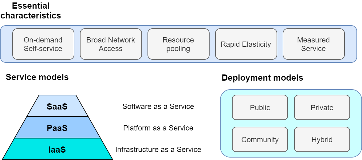
According to this, a cloud is a collection of hardware and software that meets the following requirements.
-
On-demand self-service: Computational resources are automatically allocated according to the user’s request.
-
Broad network access: Users can access the cloud through the network.
-
Resource pooling: The cloud provider allocates computational resources to multiple users by dividing the owned computational resources.
-
Rapid elasticity: To be able to quickly expand or reduce computational resources according to the user’s request.
-
Measured service: To be able to measure and monitor the amount of computing resources used.
This may sound too abstract for you to understand. Let’s talk about it in more concrete terms.
If you wanted to upgrade the CPU on your personal computer, you would have to physically open the chassis, expose the CPU socket, and replace it with a new CPU. Or, if the storage is full, you will need to remove the old disk and insert a new one. When the computer is moved to a new location, it will not be able to connect to the network until the LAN cable of the new room is plugged in.
In the cloud, these operations can be performed by commands from a program. If you want 1000 CPUs, you can send a request to the cloud provider. Within a few minutes, you will be allocated 1000 CPUs. If you want to expand your storage from 1TB to 10TB, you can send such command (you may be familiar with this from services such as Google Drive or Dropbox). When you are done using the compute resources, you can tell the provider about it, and the allocation will be deleted immediately. The cloud provider accurately monitors the amount of computing resources used, and calculates the usage fee based on that amount.
Namely, the essence of the cloud is the virtualization and abstraction of physical hardware, and users can manage and operate physical hardware through commands as if it were a part of software. Of course, behind the scenes, a huge number of computers in data centers are running, consuming a lot of power. The cloud provider achieves this virtualization and abstraction by cleverly managing the computational resources in the data center and providing the user with a software interface. From the cloud provider’s point of view, they are able to maximize their profit margin by renting out computers to a large number of users and keeping the data center utilization rate close to 100% at all times.
In the author’s words, the key characteristics of the cloud can be defined as follows:
The cloud is an abstraction of computing hardware. In other words, it is a technology that makes it possible to manipulate, expand, and connect physical hardware as if it were part of software.
Coming back to The NIST Definition of Cloud Computing mentioned above, the following three forms of cloud services are defined (Figure 2).
-
Software as a Service (SaaS)
A form of service that provides users with application running in the cloud. Examples include Google Drive and Slack. The user does not directly touch the underlying cloud infrastructure (network, servers, etc.), but use the cloud services provided as applications.
-
Platform as a Service (PaaS)
A form of service that provides users with an environment for deploying customer-created applications (which in most cases consist of a database and server code for processing API requests). In PaaS, the user does not have direct access to the cloud infrastructure, and the scaling of the server is handled by the cloud provider. Examples include Google App Engine and Heroku.
-
Infrastructure as a Service (IaaS)
A form of service that provides users with actual cloud computing infrastructure on a pay-as-you-go basis. The users rent the necessary network, servers, and storage from the provider, and deploy and operate their own applications on it. An example of IaaS is AWS EC2.
This book mainly deals with cloud development in IaaS. In other words, it is cloud development in which the developer directly manipulates the cloud infrastructure, configures the desired network, server, and storage from scratch, and deploys the application on it. In this sense, cloud development can be divided into two steps: the step of building a program that defines the cloud infrastructure and the step of crafting an application that actually runs on the infrastructure. These two steps can be separated to some extent as a programmer’s skill set, but an understanding of both is essential to build the most efficient and optimized cloud system. This book primarily focuses on the former (operating the cloud infrastructure), but also covers the application layer. PaaS is a concept where the developer focuses on the application layer development and relies on the cloud provider for the cloud infrastructure. PaaS reduces development time by eliminating the need to develop the cloud infrastructure, but has the limitation of not being able to control the detailed behavior of the infrastructure. This book does not cover PaaS techniques and concepts.
SaaS can be considered a development "product" in the context of this book. In other words, the final goal of development is to provide a computational service or database on the available to the general public by deploying the programs on IaaS platform. As a practical demonstration, we will provide hands-on exercises such as creating a simple SNS (Section 13).
Recently, Function as a Service (FaaS) and serverless computing have been recognized as new cloud categories. These concepts will be discussed in detail in later chapters (Section 12). As will become clear as you read through this book, cloud technology is constantly and rapidly evolving. This book first touches on traditional cloud design concepts from a practical and educational point of view, and then covers the latest technologies such as serverless.
Finally, according to The NIST Definition of Cloud Computing, the following four types of cloud deployment model are defined (Figure 2). Private cloud is a cloud used only within a specific organization, group, or company. For example, universities and research institutes often operate large-scale computer servers for their members. In a private cloud, any member of the organization can run computations for free or at a very low cost. However, the upper limit of available computing resources is often limited, and there may be a lack of flexibility when expanding.
Pubclic cloud is a cloud that is offered as a commercial service to general customers. Examples of famous public cloud platforms include Google Cloud Platform (GCP) provided by Google, Azure provided by Microsoft, and Amazon Web Services (AWS) provided by Amazon. When you use a public cloud, you pay the usage cost set by the provider. In return, you get access to the computational resources of the company operating the huge data center, so it is not an exaggeration to say that the computational capacity is inexhaustible.
The third type of cloud operation is called community cloud. This refers to a cloud that is shared and operated by groups and organizations that share the same objectives and roles, such as government agencies. Finally, there is the hybrid cloud, which is a cloud composed of a combination of private, public, and community clouds. An example of hybrid cloud would be a case where some sensitive and privacy-related information is kept in the private cloud, while the rest of the system depends on the public cloud.
This book is basically about cloud development using public clouds. In particular, we will use Amazon Web Services (AWS) to learn specific techniques and concepts. Note, however, that techniques such as server scaling and virtual computing environments are common to all clouds, so you should be able to acquire knowledge that is generally applicable regardless of the cloud platform.
2.2. Why use the cloud?
As mentioned above, the cloud is a computational environment where computational resources can be flexibly manipulated through programs. In this section, we would like to discuss why using the cloud is better than using a real local computing environment.
-
Scalable server size
When you start a new project, it’s hard to know in advance how much compute capacity you’ll ever need. Buying a large server is risky. On the other hand, a server that is too small can be troublesome to upgrade later on. By using the cloud, you can secure the right amount of computing resources you need as you proceed with your project.
-
Free from hardware maintainance
Sadly, computers do get old. With the rate at which technology is advancing these days, after five years, even the newest computers of the day are no more than fossils. Replacing the server every five years would be a considerable hassle. It is also necessary to deal with unexpected failures such as power outages and breakdowns of servers. With cloud computing, there is no need for the user to worry about such things, as the provider automatically takes care of the infrastructure maintenance.
-
Zero initial cost
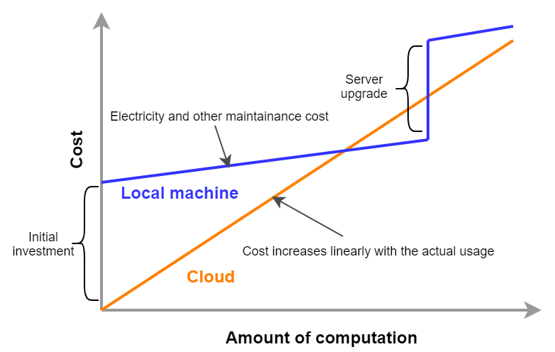
Figure 3 shows the economic cost of using your own computing environment versus the cloud. The initial cost of using the cloud is basically zero. After that, the cost increases according to the amount of usage. On the other hand, a large initial cost is incurred when using your own computing environment. After the initial investment, the increase in cost is limited to electricity and server maintenance costs, so the slope is smaller than in the case of using the cloud. Then, after a certain period of time, there may be step-like expenditures for server upgrades. The cloud, on the other hand, incur no such discontinuous increase in cost. In the areas where cost curve of the cloud is below that of local computing environment, using the cloud will lead to economic cost savings.
In particular, point 1 is important in research situations. In research, there are few cases in which one must keep running computations all the time. Rather, the computational load is likely to increase intensively and unexpectedly when a new algorithm is conceived, or when new data arrives. In such cases, the ability to flexibly increase computing power is a major advantage of using the cloud.
So far, we have discussed the advantages of using the cloud, but there are also some disadvantages.
-
The cloud must be used wisely
As shown in the cost curve in Figure 3, depending on your use case, there may be situations where it is more cost effective to use local computing environment. When using the cloud, users are required to manage their computing resources wisely, such as deleting intances immediately after use.
-
Security
The cloud is accessible from anywhere in the world via the Internet, and can be easily hacked if security management is neglected. If the cloud is hacked, not only will information be leaked, but there is also the possibility of financial loss.
-
Learning Curve
As described above, there are many points to keep in mind when using the cloud, such as cost and security. In order to use the cloud wisely, it is indispensable to have a good understanding of the cloud and to overcome the learning curve.
The black screen that you use to enter commands on Mac or Linux is called a terminal. Do you know the origin of this word?
The origin of this word goes back to the early days of computers. At that time, a computer was a machine the size of a conference room, with thousands of vacuum tubes connected together. Since it was such an expensive and complex piece of equipment, it was natural that it would be shared by many people. In order for users to access the computer, there were several cables running from the machine, each with a keyboard and screen attached to it… This was called a Terminal. People took turns sitting in front of the terminal and interacting with the computer.
Times change, and with the advent of personal computers such as Windows and Mac, computers have become something that is owned by individuals rather than shared by everyone.
The recent rise of cloud computing can be seen as a return to the original usage of computers, where everyone shared a large computer. At the same time, edge devices such as smartphones and wearables are becoming more and more popular, and the trend of individuals owning multiple "small" computers is progressing at the same time.
3. Introduction to AWS
3.1. What is AWS?
In this book, AWS is used as the platform for implementing cloud applications. In this chapter, we will explain the essential knowledge of AWS that is required for hands-on tutorials.
AWS (Amazon Web Services) is a general cloud platform provided by Amazon. AWS was born in 2006 as a cloud service that leases vast computing resources that Amazon owns. In 2021, AWS holds the largest market share (about 32%) as a cloud provider (Ref). Many web-related services, including Netflix and Slack, have some or all of their server resources provided by AWS. Therefore, most of the readers would be benefiting from AWS without knowing it.
Because it has the largest market share, it offers a wider range of functions and services than any other cloud platforms. In addition, reflecting the large number of users, there are many official and third-party technical articles on the web, which is helpful in learning and debugging. In the early days, most of the users were companies engaged in web business, but recently, there is a growing number of users embracing AWS for scientific and engineering research.
3.2. Functions and services provided by AWS
Figure 4 shows a list of the major services provided by AWS at the time of writing.
The various elements required to compose a cloud, such as computation, storage, database, network, and security, are provided as independent components. Essentially, a cloud system is created by combining these components. There are also pre-packaged services for specific applications, such as machine learning, speech recognition, and augmented reality (AR) and virtual reality (VR). In total, there are more than 170 services provided.
AWS beginners often fall into a situation where they are overwhelmed by the large number of services and left at a loss. It’s not even clear what concepts to learn and in what order, and this is undoubtedly a major barrier to entry. However, the truth is that the essential components of AWS are limited to just a couple. If you know how to use the essential components, you are almost ready to start developing on AWS. Many of the other services are combinations of the basic elements that AWS has prepared as specialized packages for specific applications. Recognizing this point is the first step in learning AWS.
Here, we list the essential components for building a cloud system on AWS. You will experience them while writing programs in the hands-on sessions in later chapters. At this point, it is enough if you could just memorize the names in a corner of your mind.
3.2.1. computation
![]() EC2 (Elastic Compute Cloud)
Virtual machines with various specifications can be created and used to perform calculations.
This is the most basic component of AWS.
We will explore more on EC2 in later chapters (Section 4, Section 6, Section 9).
EC2 (Elastic Compute Cloud)
Virtual machines with various specifications can be created and used to perform calculations.
This is the most basic component of AWS.
We will explore more on EC2 in later chapters (Section 4, Section 6, Section 9).
![]() Lambda
Lambda is a part of the cloud called Function as a Service (FaaS), a service for performing small computations without a server.
It will be described in detail in the chapter on serverless architecture (Section 11).
Lambda
Lambda is a part of the cloud called Function as a Service (FaaS), a service for performing small computations without a server.
It will be described in detail in the chapter on serverless architecture (Section 11).
3.2.2. Storage
![]() EBS (Elastic Block Store)
A virtual data drive that can be assigned to EC2.
Think of a "conventional" file system as used in common operating systems.
EBS (Elastic Block Store)
A virtual data drive that can be assigned to EC2.
Think of a "conventional" file system as used in common operating systems.
![]() S3 (Simple Storage Service)
S3 is a "cloud-bative" data storage system called Object Storage, which uses APIs to read and write data.
It will be described in detail in the chapter on serverless architecture (Section 11).
S3 (Simple Storage Service)
S3 is a "cloud-bative" data storage system called Object Storage, which uses APIs to read and write data.
It will be described in detail in the chapter on serverless architecture (Section 11).
3.2.3. Database
![]() DynamoDB
DynamoDB is a NoSQL type database service (think of
DynamoDB
DynamoDB is a NoSQL type database service (think of mongoDB if you know it).
It will be described in detail in the chapter on serverless architecture (Section 11).
3.2.4. Networking
![]() VPC(Virtual Private Cloud)
With VPC, one can create a virtual network environment on AWS, define connections between virtual servers, and manage external access.
EC2 must be placed inside a VPC.
VPC(Virtual Private Cloud)
With VPC, one can create a virtual network environment on AWS, define connections between virtual servers, and manage external access.
EC2 must be placed inside a VPC.
API Gateway
![]() API Gateway acts as a reverse proxy to connect API endpoints to backend services (such as Lambda).
It will be described in detail in Section 13.
API Gateway acts as a reverse proxy to connect API endpoints to backend services (such as Lambda).
It will be described in detail in Section 13.
3.3. Regions and Availability Zones
One of the most important concepts you need to know when using AWS is Region and Availability Zone (AZ) (Figure 5). In the following, we will briefly describe these concepts. For more detailed information, also see official documentation "Regions, Availability Zones, and Local Zones".
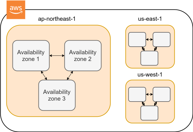
A region roughly means the location of a data center.
At the time of writing, AWS has data centers in 25 geographical locations around the world, as shown in Figure 6.
In Japan, there are data centers in Tokyo and Osaka.
Each region has a unique ID, for example, Tokyo is defined as ap-northeast-1, Ohio as us-east-2, and so on.

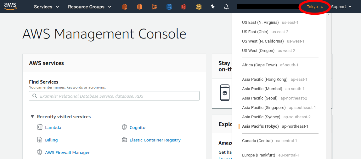
When you log in to the AWS console, you can select a region from the menu bar at the top right of the screen (Figure 7, circled in red). AWS resources such as EC2 are completely independent for each region. Therefore, when deploying new resources or viewing deployed resources, you need to make sure that the console region is set correctly. If you are developing a web business, you will need to deploy the cloud in various parts of the world. However, if you are using it for personal research, you are most likely fine just using the nearest region (e.g. Tokyo).
An Avaialibity Zone (AZ) is a data center that is geographically isolated within a region. Each region has two or more AZs, so that if a fire or power failure occurs in one AZ, the other AZs can cover the failure. In addition, the AZs are connected to each other by high-speed dedicated network lines, so data transfer between AZs is extremely fast. AZ is a concept that should be taken into account when server downtime is unacceptable, such as in web businesses. For personal use, there is no need to be concerned much about it. It is sufficient to know the meaning of the term.
|
When using AWS, which region should you select? In terms of Internet connection speed, it is generally best to use the region that is geographically closest to you. On the other hand, EC2 usage fees, etc., are priced slightly differently for each region. Therefore, it is also important to choose the region with the lowest price for the services that you use most frequently. In addition, some services may not be available in a particular region. It is best to make an overall judgment based on these points. |
3.4. Cloud development in AWS
Now that you have a general understanding of the AWS cloud, the next topic will be an overview of how to develop and deploy a cloud system on AWS.
There are two ways to perform AWS operations such as adding, editing, and deleting resources: using the console and using the API.
3.4.1. Operating the resources through the console
When you log in to your AWS account, the first thing you will see is the AWS Management Console (Figure 8).
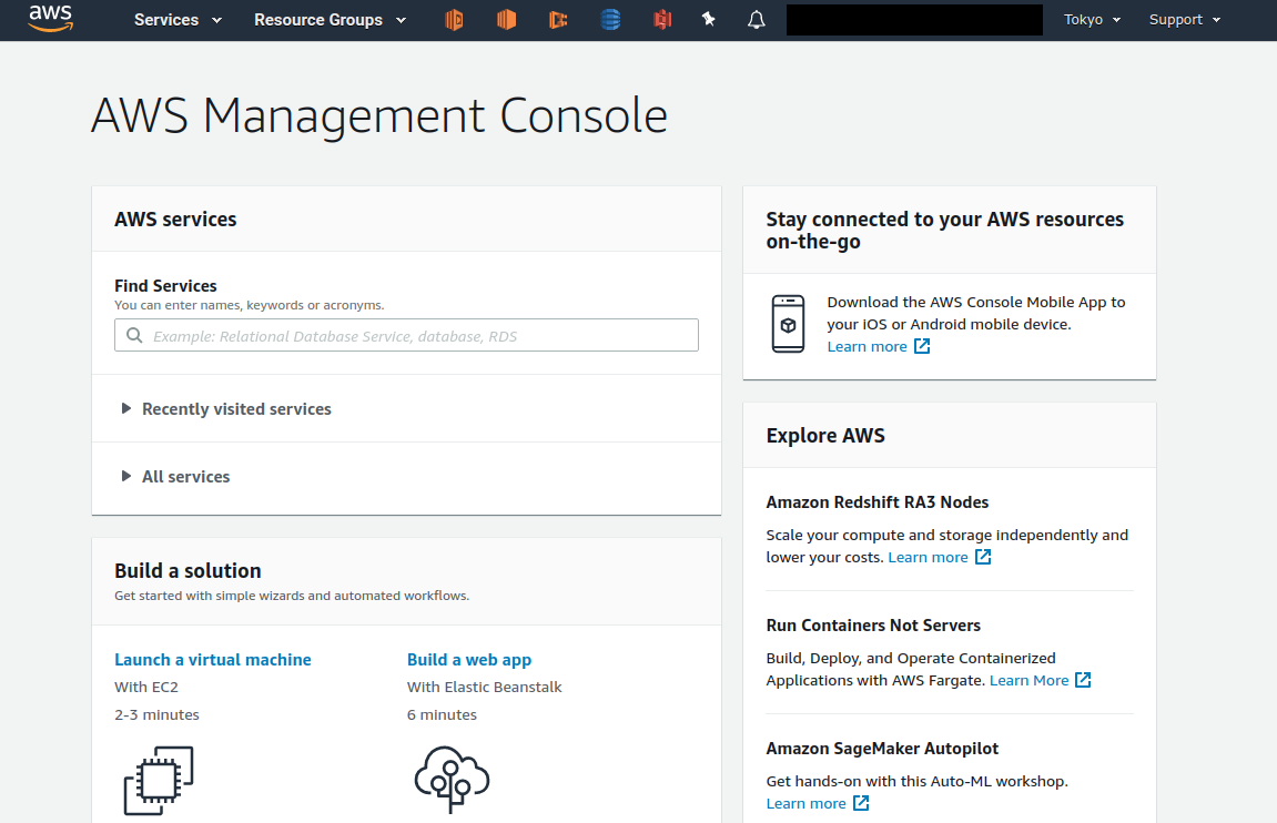
|
In this book we will often call AWS Management Console AWS console or just a console. |
Using the console, you can peform any operations on AWS resources through a GUI (Graphical User Interface), such as launching EC2 instances, adding and deleting data in S3, viewing logs, and so on. AWS console is very useful when you are trying out a new function for the first time or debugging the system.
The console is useful for quickly testing functions and debugging the cloud under development, but it is rarely used directly in actual cloud development. Rather, it is more common to use the APIs to describe cloud resources programmatically. For this reason, this book does not cover how to use AWS console. The AWS documentation includes many tutorials which describe how to perform various operations from the AWS console. They are valuable resources for learning.
3.4.2. Operating the resources through the APIs
By using API (Application Programming Interface), you can send commands to AWS and manipulate cloud resources. APIs are simply a list of commands exposed by AWS, and consisted of REST APIs (REST APIs are explained in Section 10.2). However, directly entering the REST APIs can be tedious, so various tools are provided to interact with AWS APIs more conveniently.
For example, AWS CLI is a command line interface (CLI) to execute AWS APIs through UNIX console. In addition to the CLI, SDKs (Software Development Kits) are available in a variety of programming languages. Some examples are listed below.
-
Python ⇒ boto3
-
Ruby ⇒ AWS SDK for Ruby
-
Node.js ⇒ AWS SDK for Node.js
Let’s look at a some of the API examples.
Let’s assume that you want to add a new storage space (called a Bucket) to S3.
If you use the AWS CLI, you can type a command like the following.
$ aws s3 mb s3://my-bucket --region ap-northeast-1The above command will create a bucket named my-bucket in the ap-northeast-1 region.
To perform the same operation from Python, use the boto3 library and run a script like the following.
1
2
3
4
import boto3

s3_client = boto3.client("s3", region_name="ap-northeast-1")
s3_client.create_bucket(Bucket="my-bucket")
Let’s look at another example.
To start a new EC2 instance (an instance is a virtual server that is in the running state), use the following command.
$ aws ec2 run-instances --image-id ami-xxxxxxxx --count 1 --instance-type t2.micro --key-name MyKeyPair --security-group-ids sg-903004f8 --subnet-id subnet-6e7f829eThis command will launch a t2.micro instance with 1 vCPU and 1.0 GB RAM. We’ll explain more about this command in later chapter (Section 4).
To perform the same operation from Python, use a script like the following.
 1
 2
 3
 4
 5
 6
 7
 8
 9
10
11
12
import boto3

ec2_client = boto3.client("ec2")
ec2_client.run_instances(
    ImageId="ami-xxxxxxxxx",
    MinCount=1,
    MaxCount=1,
    KeyName="MyKeyPair",
    InstanceType="t2.micro",
    SecurityGroupIds=["sg-903004f8"],
    SubnetId="subnet-6e7f829e",
)
Through the above examples, we hope you are starting to get an idea of how APIs can be used to manipulate cloud resources. With a single command, you can start a new virtual server, add a data storage area, or perform any other operation you want. By combining multiple commands like this, you can build a computing environment with the desired CPU, RAM, network, and storage. Of course, the delete operation can also be performed using the API.
3.4.3. Mini hands-on: Using AWS CLI
In this mini hands-on, we will learn how to use AWS CLI.
As mentioned earlier, AWS CLI can be used to manipulate any resource on AWS, but here we will practice the simplest case, reading and writing files using S3.
(EC2 operations are a bit more complicated, so we will cover them in Section 4).
For detailed usage of the aws s3 command, please refer to official documentation.
|
For information on installing the AWS CLI, see Section 14.3. |
|
The hands-on exercise described below can be performed within the free S3 tier. |
|
Before executing the following commands, make sure that your AWS credentials are set correctly.
This requires that the settings are written to the file |
To begin with, let’s create a data storage space (called a Bucket) in S3.
$ bucketName="mybucket-$(openssl rand -hex 12)"
$ echo $bucketName
$ aws s3 mb "s3://${bucketName}"
Since the name of an S3 bucket must be unique across AWS, the above command generates a bucket name that contains a random string and stores it in a variable called bucketName.
Then, a new bucket is created by aws s3 mb command (mb stands for make bucket).
Next, let’s obtain a list of the buckets.
$ aws s3 ls

2020-06-07 23:45:44 mybucket-c6f93855550a72b5b66f5efe
We can see that the bucket we just created is in the list.
|
As a notation in this book, terminal commands are prefixed with |
Next, we upload the files to the bucket.
$ echo "Hello world!" > hello_world.txt
$ aws s3 cp hello_world.txt "s3://${bucketName}/hello_world.txt"
Here, we generated a dummy file hello_world.txt and uploaded it to the bucket.
Now, let’s obtain a list of the files in teh bucket.
$ aws s3 ls "s3://${bucketName}" --human-readable

2020-06-07 23:54:19   13 Bytes hello_world.txt
We can see that the file we just uploaded is in the list.
Lastly, we delete the bucket we no longer use.
$ aws s3 rb "s3://${bucketName}" --forcerb stands for remove bucket.
By default, you cannot delete a bucket if there are files in it.
By adding the --force option, a non-empty bucket are forced to be deleted.
As we just saw, we were able to perform a series of operations on S3 buckets using the AWS CLI. In the same manner, you can use the AWS CLI to perform operation on EC2, Lambda, DynamoDB, and any other resources.
|
Amazon Resource Name (ARN). Every resource on AWS is assigned a unique ID called Amazon Resource Name (ARN).
ARNs are written in a format like In addition to ARNs, it is also possible to define human-readable names for S3 buckets and EC2 instances. In this case, either the ARN or the name can be used to refer to the same resource. |
3.5. CloudFormation and AWS CDK
As mentioned in the previous section, AWS APIs can be used to create and manage any resources in the cloud. Therefore, in principle, you can construct cloud systems by combining API commands.
However, there is one practical point that needs to be considered here. The AWS API can be broadly divided into commands to manipulate resources and commands to execute tasks (Figure 9).
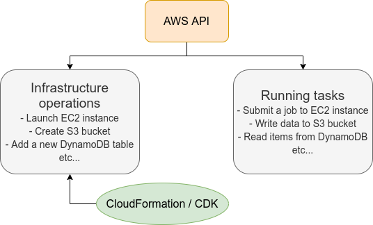
Manipulating resources refers to preparing static resources, such as launching an EC2 instance, creating an S3 bucket, or adding a new table to a database. Such commands need to be executed only once, when the cloud is deployed.
Commands to execute tasks refer to operations such as submitting a job to an EC2 instance or writing data to an S3 bucket. It describes the computation that should be performed within the premise of a static resource such as EC2 instance or S3 bucket. Compared to the former, the latter can be regarded as being in charge of dynamic operations.
From this point of view, it would be clever to manage programs describing the infrastructure and programs executing tasks separately. Therefore, the development of a cloud can be divided into two steps: one is to create programs that describe the static resources of the cloud, and the other is to create programs that perform dynamic operations.
CloudFormation is a mechanism for managing static resources in AWS. CloudFormation defines the blueprint of the cloud infrastructure using text files that follow the CloudFormation syntax. CloudFormation can be used to describe resource requirements, such as how many EC2 instances to launch, with what CPU power and networks configuration, and what access permissions to grant. Once a CloudFormation file has been crafted, a cloud system can be deployed on AWS with a single command. In addition, by exchanging CloudFormation files, it is possible for others to easily reproduce an identical cloud system. This concept of describing and managing cloud infrastructure programmatically is called Infrastructure as Code (IaC).
CloudFormation usually use a format called JSON (JavaScript Object Notation). The following code is an example excerpt of a CloudFormation file written in JSON.
 1
 2
 3
 4
 5
 6
 7
 8
 9
10
11
12
13
14
15
16
17
18
19
20
21
22
23
24
25
26
27
28
29
30
"Resources" : {
  ...
  "WebServer": {
    "Type" : "AWS::EC2::Instance",
    "Properties": {
      "ImageId" : { "Fn::FindInMap" : [ "AWSRegionArch2AMI", { "Ref" : "AWS::Region" },
                        { "Fn::FindInMap" : [ "AWSInstanceType2Arch", { "Ref" : "InstanceType" }, "Arch" ] } ] },
      "InstanceType"   : { "Ref" : "InstanceType" },
      "SecurityGroups" : [ {"Ref" : "WebServerSecurityGroup"} ],
      "KeyName"        : { "Ref" : "KeyName" },
      "UserData" : { "Fn::Base64" : { "Fn::Join" : ["", [
                     "#!/bin/bash -xe\n",
                     "yum update -y aws-cfn-bootstrap\n",

                     "/opt/aws/bin/cfn-init -v ",
                     "         --stack ", { "Ref" : "AWS::StackName" },
                     "         --resource WebServer ",
                     "         --configsets wordpress_install ",
                     "         --region ", { "Ref" : "AWS::Region" }, "\n",

                     "/opt/aws/bin/cfn-signal -e $? ",
                     "         --stack ", { "Ref" : "AWS::StackName" },
                     "         --resource WebServer ",
                     "         --region ", { "Ref" : "AWS::Region" }, "\n"
      ]]}}
    },
    ...
  },
  ...
},
Here, we have defined an EC2 instance named "WebServer". This is a rather long and complex description, but it specifies all necessary information to create an EC2 instance.
3.5.1. AWS CDK
As we saw in the previous section, CloudFormation is very complex to write, and there must not be any errors in any lines. Further, since CloudFormation is written with JSON, we cannot use useful concepts such as variables and classes as we do in modern programming languages (strictly speaking, CloudFormation has functions that are equivalent to variables). In addition, many parts of the CloudFormation files are repetitive, and many parts can be automated.
To solve this programmer’s pain, AWS Cloud Development Kit (CDK) is offered by AWS. CDK is a tool that automatically generates CloudFormations using a programming language such as Python. CDK is a relatively new tool, released in 2019, and is being actively developed (check the releases at GitHub repository to see how fast this library is being improved). CDK is supported by several languages including TypeScript (JavaScript), Python, and Java.
With CDK, programmers can use a familiar programming language to describe the deisred cloud resources and synthesize the CloudFormation files. In addition, CDK determines many of the common parameters automatically, which reduces the amount of coding.
The following is an example excerpt of CDK code using Python.
 1
 2
 3
 4
 5
 6
 7
 8
 9
10
11
12
13
14
15
16
17
18
19
20
21
22
23
24
25
26
import aws_cdk as cdk
from aws_cdk import (
    Stack,
    aws_ec2 as ec2,
)

class MyFirstEc2(Stack):

    def __init__(self, scope, construct_id, **kwargs):
        super().__init__(scope, construct_id, **kwargs)

        vpc = ec2.Vpc(
            ... # some parameters
        )

        sg = ec2.SecurityGroup(
            ... # some parameters
        )

        host = ec2.Instance(
            self, "MyGreatEc2",
            instance_type=ec2.InstanceType("t2.micro"),
            machine_image=ec2.MachineImage.latest_amazon_linux(),
            vpc=vpc,
            ...
        )
This code describes essentially the same thing as the JSON-based CloudFormation shown in the previous section. You can see that CDK code is much shorter and easier to understand than the very complicated CloudFormation file.
The focus of this book is to help you learn AWS concepts and techniques while writing code using CDK. In the later chapters, we will provide various hands-on exercises using CDK. To kick start, in the first hands-on, we will learn how to launch a simple EC2 instance using CDK.
4. Hands-on #1: Launching an EC2 instance
In the first hands-on session, we will create an EC2 instance (virtual server) using CDK, and log in to the server using SSH. After this hands-on, you will be able to set up your own server on AWS and run calculations as you wish!
4.1. Preparation
The source code for the hands-on is available on GitHub at handson/ec2-get-started.
|
This hands-on exercise can be performed within the free EC2 tier. |
First, we set up the environment for the exercise. This is a prerequisite for the hands-on sessions in later chapters as well, so make sure to do it now without mistakes.
-
AWS account: You will need a personal AWS account to run the hands-on. See Section 14.1 for obtaining an AWS account.
-
Python and Node.js: Python (3.6 or higher) and Node.js (12.0 or higher) must be installed in order to run this hands-on.
-
AWS CLI: For information on installing the AWS CLI, see Section 14.3. Be sure to set up the authentication key described here.
-
AWS CDK: For information on installing the AWS CDK, see Section 14.4.
-
Downloading the source code: Download the source code of the hands-on program from GitHub using the following command.
$ git clone https://github.com/tomomano/learn-aws-by-coding.gitAlternatively, you can go to https://github.com/tomomano/learn-aws-by-coding and click on the download button in the upper right corner.
Using Docker image for the hands-on exercises
We provide a Docker image with the required programs installed, such as Python, Node.js, and AWS CDK. The source code of the hands-on program has also been included in the image. If you already know how to use Docker, then you can use this image to immediately start the hands-on tutorials without having to install anything else.
See Section 14.8 for more instructions.
4.2. SSH
SSH (secure shell) is a tool to securely access Unix-like remote servers. In this hands-on, we will use SSH to access a virtual server. For readers who are not familiar with SSH, here we give a brief guidance.
All SSH communication is encrypted, so confidential information can be sent and received securely over the Internet. For this hands-on, you need to have an SSH client installed on your local machine to access the remote server. SSH clients come standard on Linux and Mac. For Windows, it is recommended to install WSL to use an SSH client (see [environments]).
The basic usage of the SSH command is shown below.
<host name> is the IP address or DNS hostname of the server to be accessed.
The <user name> is the user name of the server to be connected to.
$ ssh <user name>@<host name>SSH can be authenticated using plain text passwords, but for stronger security, it is strongly recommended that you use Public Key Cryptography authentication, and EC2 only allows access in this way. We do not explain the theory of public key cryptography here. The important point in this hands-on is that the EC2 instance holds the public key, and the client computer (the reader’s local machine) holds the private key. Only the computer with the private key can access the EC2 instance. Conversely, if the private key is leaked, a third party will be able to access the server, so manage the private key with care to ensure that it is never leaked.
The SSH command allows you to specify the private key file to use for login with the -i or --identity_file option.
For example, use the following command.
$ ssh -i Ec2SecretKey.pem <user name>@<host name>4.3. Reading the application source code
Figure 10 shows an overview of the application we will be deploying in this hands-on.
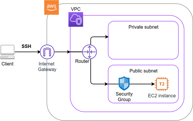
In this application, we first set up a private virtual network environment using VPC (Virtual Private Cloud). The virtual servers of EC2 (Elastic Compute Cloud) are placed inside the public subnet of the VPC. For security purposes, access to the EC2 instance is restricted by the Security Group (SG). We will use SSH to access the virtual server and perform a simple calculation. We use AWS CDK to construct this application.
Let’s take a look at the source code of the CDK app (handson/ec2-get-started/app.py).
 1
 2
 3
 4
 5
 6
 7
 8
 9
10
11
12
13
14
15
16
17
18
19
20
21
22
23
24
25
26
27
28
29
30
31
32
33
34
35
36
37
38
39
40
class MyFirstEc2(Stack):

    def __init__(self, scope: Construct, construct_id: str, key_name: str, **kwargs) -> None:
        super().__init__(scope, construct_id, **kwargs)

        (1)
        vpc = ec2.Vpc(
            self, "MyFirstEc2-Vpc",
            max_azs=1,
            ip_addresses=ec2.IpAddresses.cidr("10.10.0.0/23"),
            subnet_configuration=[
                ec2.SubnetConfiguration(
                    name="public",
                    subnet_type=ec2.SubnetType.PUBLIC,
                )
            ],
            nat_gateways=0,
        )

        (2)
        sg = ec2.SecurityGroup(
            self, "MyFirstEc2Vpc-Sg",
            vpc=vpc,
            allow_all_outbound=True,
        )
        sg.add_ingress_rule(
            peer=ec2.Peer.any_ipv4(),
            connection=ec2.Port.tcp(22),
        )

        (3)
        host = ec2.Instance(
            self, "MyFirstEc2Instance",
            instance_type=ec2.InstanceType("t2.micro"),
            machine_image=ec2.MachineImage.latest_amazon_linux(),
            vpc=vpc,
            vpc_subnets=ec2.SubnetSelection(subnet_type=ec2.SubnetType.PUBLIC),
            security_group=sg,
            key_name=key_name
        )
| 1 | First, we define the VPC. |
| 2 | Next, we define the security group. Here, connections from any IPv4 address to port 22 (used for SSH connections) are allowed. All other connections are rejected. |
| 3 | Finally, an EC2 instance is created with the VPC and SG created above.
The instance type is selected as t2.micro, and Amazon Linux is used as the OS. |
Let us explain each of these points in more detail.
4.3.1. VPC (Virtual Private Cloud)

VPC is a tool for building a private virtual network environment on AWS. In order to build advanced computing systems, it is necessary to connect multiple servers, which requires management of the network addresses. VPC is useful for such purposes.
In this hands-on, only one server is launched, so the benefits of VPC may not be clear to you. However, since AWS specification require that EC2 instances must be placed inside a VPC, we have configured a minimal VPC in this application.
|
For those who are interested, here is a more advanced explanation of the VPC code.
|
4.3.2. Security Group
A security group (SG) is a virtual firewall that can be assigned to an EC2 instance. For example, you can allow or deny connections coming from a specific IP address (inbound traffic restriction), and prohibit access to a specific IP address (outbound traffic restriction).
Let’s look at the corresponding part of the code.
1
2
3
4
5
6
7
8
9
sg = ec2.SecurityGroup(
    self, "MyFirstEc2Vpc-Sg",
    vpc=vpc,
    allow_all_outbound=True,
)
sg.add_ingress_rule(
    peer=ec2.Peer.any_ipv4(),
    connection=ec2.Port.tcp(22),
)
Here, in order to allow SSH connections from the outside, we specified sg.add_ingress_rule(peer=ec2.Peer.any_ipv4(), connection=ec2.Port.tcp(22)), which means that access to port 22 is allowed from all IPv4 addresses.
In addition, the parameter allow_all_outbound=True is set so that the instance can access the Internet freely to download resources.
|
SSH by default uses port 22 for remote access. |
|
From a security purpose, it is preferable to allow SSH connections only from specific locations such as home, university, or workplace. |
4.3.3. EC2 (Elastic Compute Cloud)

EC2 is a service for setting up virtual servers on AWS. Each virtual server in a running state is called an instance. (However, in colloquial communication, the terms server and instance are often used interchangeably.)
EC2 provides a variety of instance types to suit many use cases. Table 2 lists some representative instance types. A complete list of EC2 instance types can be found at Official Documentation "Amazon EC2 Instance Types".
| Instance | vCPU | Memory (GiB) | Network bandwidth (Gbps) | Price per hour ($) |
|---|---|---|---|---|
t2.micro |
1 |
1 |
- |
0.0116 |
t2.small |
1 |
2 |
- |
0.023 |
t2.medium |
2 |
4 |
- |
0.0464 |
c5.24xlarge |
96 |
192 |
25 |
4.08 |
c5n.18xlarge |
72 |
192 |
100 |
3.888 |
x1e.16xlarge |
64 |
1952 |
10 |
13.344 |
As can be seen in Table 2, the virtual CPUs (vCPUs) can be configured from 1 to 96 cores, memory from 1GB to over 2TB, and network bandwidth up to 100Gbps.
The price per hour increases approximately linearly with the number of vCPUs and memories allocated.
EC2 keeps track of the server running time in seconds, and the usage fee is determined in proportion to the usage time.
For example, if an instance of t2.medium is launched for 10 hours, a fee of 0.0464 * 10 = $0.464 will be charged.
|
AWS has a
free EC2 tier.
With this, |
|
The price listed in Table 2 is for the |
|
The above price of $0.0116 / hour for t2.micro is for the on-demand instance type. In addition to on-demand instance type, there is another type of instance called spot instance. The idea of spot instances is to rent out the excess free CPUs temporarily available at AWS data center to users at a discount. Therefore, spot instances are offered at a much lower price, but the instance may be forcibly shut down when the load on the AWS data center increases, even if the user’s program is still running. There have been many reports of spot instance being used to reduce costs in applications such as scientific computing and web servers. |
Let’s take a look at the part of the code that defines the EC2 instance.
1
2
3
4
5
6
7
8
9
host = ec2.Instance(
    self, "MyFirstEc2Instance",
    instance_type=ec2.InstanceType("t2.micro"),
    machine_image=ec2.MachineImage.latest_amazon_linux(),
    vpc=vpc,
    vpc_subnets=ec2.SubnetSelection(subnet_type=ec2.SubnetType.PUBLIC),
    security_group=sg,
    key_name=key_name
)
Here, we have selected the instance type t2.micro.
In addition, the machine_image is set to
Amazon Linux
(Machine image is a concept similar to OS.
We will discuss machine image in more detail in Section 6.)
In addition, the VPC and SG defined above are assigned to this instance.
This is a brief explanation of the program we will be using. Although it is a minimalist program, we hope it has given you an idea of the steps required to create a virtual server.
4.4. Deploying the application
Now that we understand the source code, let’s deploy the application on AWS. Again, it is assumed that you have finished the preparations described inSection 4.1.
4.4.1. Installing Python dependencies
The first step is to install the Python dependency libraries. In the following, we use venv as a tool to manage Python libraries.
First, let’s move to the directory handson/ec2-get-started.
$ cd handson/ec2-get-startedAfter moving the directory, create a new virtual environment with venv and run the installation with pip.
$ python3 -m venv .env
$ source .env/bin/activate
$ pip install -r requirements.txt
This completes the Python environment setup.
|
A quick tutorial on |
4.4.2. Setting AWS access key
To use the AWS CLI and AWS CDK, you need to have an AWS access key set up. Refer to Section 14.2 for issuing a access key. After issuing the access key, refer to Section 14.3 to configure the command line settings.
To summarize the procedure shortly, the first method is to set environment variables such as AWS_ACCESS_KEY_ID.
The second method is to store the authentication information in ~/.aws/credentials.
Setting an access key is a common step in using the AWS CLI/CDK, so make sure you understand it well.
4.4.3. Generating a SSH key pair
We login to the EC2 instance using SSH. Before creating an EC2 instance, you need to prepare an SSH public/private key pair to be used exclusively in this hands-on exercise.
Using the following AWS CLI command, let’s generate a key named OpenSesame.
$ export KEY_NAME="OpenSesame"
$ aws ec2 create-key-pair --key-name ${KEY_NAME} --query 'KeyMaterial' --output text > ${KEY_NAME}.pem
When you execute this command, a file named OpenSesame.pem will be created in the current directory.
This is the private key to access the server.
To use this key with SSH, move the key to the directory ~/.ssh/.
To prevent the private key from being overwritten or viewed by a third party, you must set the access permission of the file to 400.
$ mv OpenSesame.pem ~/.ssh/
$ chmod 400 ~/.ssh/OpenSesame.pem
4.4.4. Deploy
We are now ready to deploy our EC2 instance!
Use the following command to deploy the application on AWS.
The option -c key_name="OpenSesame" specifies to use the key named OpenSesame that we generated earlier.
$ cdk deploy -c key_name="OpenSesame"When this command is executed, the VPC, EC2, and other resources will be deployed on AWS.
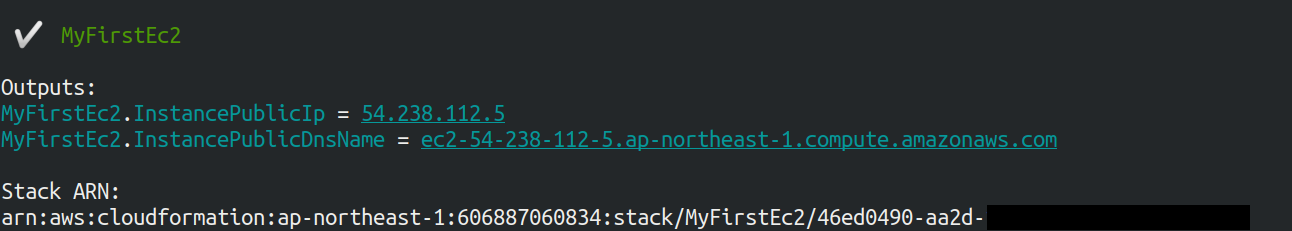
At the end of the command output, you should get an output like Figure 11.
In the output, the digits following InstancePublicIp is the public IP address of the launched instance.
The IP address is randomly assigned for each deployment.
4.4.5. Log in with SSH
Let us log in to the instance using SSH.
$ ssh -i ~/.ssh/OpenSesame.pem ec2-user@<IP address>Note that the -i option specifies the private key that was generated earlier.
Since the EC2 instance by default has a user named ec2-user, use this as a login user name.
Lastly, replace <IP address> with the IP address of the EC2 instance you created (e.g., 12.345.678.9).
If the login is successful, you will be taken to a terminal window like Figure 12.
Since you are logging in to a remote server, make sure the prompt looks like [ec2-user@ip-10-10-1-217 ~]$.
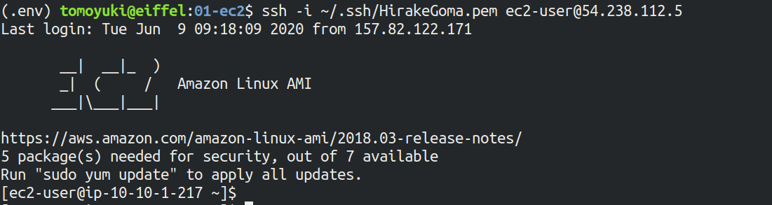
Congratulations! You have successfully launched an EC2 virtual instance on AWS, and you can access it remotely!
4.4.6. Exploring the launched EC2 instance
Now that we have a new instance up and running, let’s play with it.
Inside the EC2 instance you logged into, run the following command. The command will output the CPU information.
$ cat /proc/cpuinfo
processor : 0
vendor_id : GenuineIntel
cpu family : 6
model : 63
model name : Intel(R) Xeon(R) CPU E5-2676 v3 @ 2.40GHz
stepping : 2
microcode : 0x43
cpu MHz : 2400.096
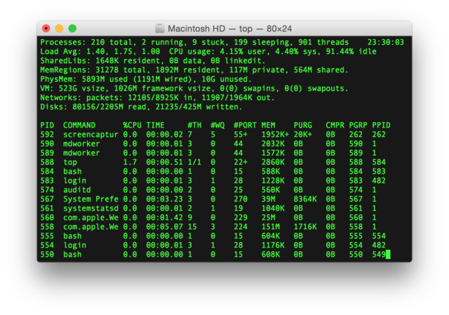
cache size : 30720 KBNext, let’s use top command and show the running processes and memory usage.
$  top -n 1

top - 09:29:19 up 43 min,  1 user,  load average: 0.00, 0.00, 0.00
Tasks:  76 total,   1 running,  51 sleeping,   0 stopped,   0 zombie
Cpu(s):  0.3%us,  0.3%sy,  0.1%ni, 98.9%id,  0.2%wa,  0.0%hi,  0.0%si,  0.2%st
Mem:   1009140k total,   270760k used,   738380k free,    14340k buffers
Swap:        0k total,        0k used,        0k free,   185856k cached

  PID USER      PR  NI  VIRT  RES  SHR S %CPU %MEM    TIME+  COMMAND
    1 root      20   0 19696 2596 2268 S  0.0  0.3   0:01.21 init
    2 root      20   0     0    0    0 S  0.0  0.0   0:00.00 kthreadd
    3 root      20   0     0    0    0 I  0.0  0.0   0:00.00 kworker/0:0
Since we are using t2.micro instance, we have 1009140k = 1GB memory in the virtual instance.
The instance we started has Python 2 installed, but not Python 3. Let’s install Python 3.6. The installation is easy.
$ sudo yum update -y
$ sudo yum install -y python36
Let’s start Python 3 interpreter.
$ python3
Python 3.6.10 (default, Feb 10 2020, 19:55:14)
[GCC 4.8.5 20150623 (Red Hat 4.8.5-28)] on linux
Type "help", "copyright", "credits" or "license" for more information.
>>>
To exit from the interpreter, use Ctrl + D or type exit().
So, that’s it for playing around on the server (if you’re interested, you can try different things!). Log out from the instance with the following command.
$ exit4.4.7. Observing the resources from AWS console
So far we have performed all EC2-related operations from the command line. Operations such as checking the status of an EC2 instance or shutting down a server can also be performed from the AWS console. Let’s take a quick look at this.
First, open a web browser and log in to the AWS console.
Once you are logged in, search EC2 from Services and go to the EC2 dashboard.
Next, navigate to Instances in the left sidebar.
You should get a screen like Figure 13.
On this screen, you can check the instances under your account.
Similarly, you can also check the VPC and SG from the console.
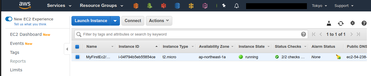
|
Make sure that the correct region (in this case, |
As mentioned in the previous chapter, the application deployed here is managed as a CloudFormation stack.
A stack refers to a group of AWS resources.
In this case, VPC, SG, and EC2 are included in the same stack.
From the AWS console, let’s go to the CloudFormation dashboard (Figure 14).
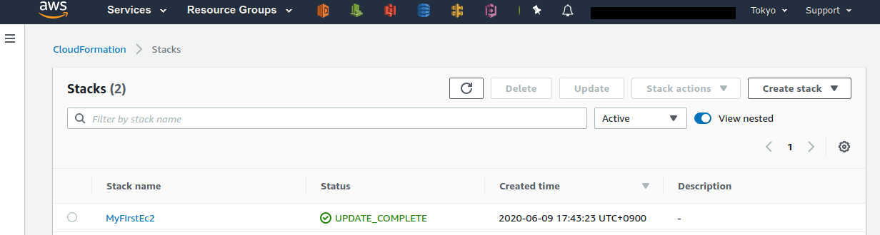
You should be able find a stack named "MyFirstEc2". If you click on it and look at the contents, you will see that EC2, VPC, and other resources are associated to this stack.
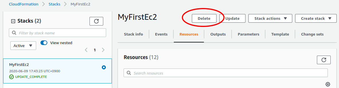
4.4.8. Deleting the stack
We have explained everything that was to be covered in the first hands-on session. Finally, we must delete the stack that is no longer in use. There are two ways to delete a stack.
The first method is to press the "Delete" button on the Cloudformation dashboard (Figure 15).
Then, the status of the stack will change to "DELETE_IN_PROGRESS", and when the deletion is completed, the stack will disappear from the list of CloudFormation stacks.
The second method is to use the command line. Let’s go back to the command line where we ran the deployment. Then, execute the following command.
$ cdk destroyWhen you execute this command, the stack will be deleted. After deleting the stack, make sure for yourself that all the VPCs, EC2s, etc. have disappeared without a trace. Using CloudFormation is very convenient because it allows you to manage and delete all related AWS resources at once.
|
Make sure you delete your own stack! If you do not do so, you will continue to be charged for the EC2 instance! |
Also, delete the SSH key pair created for this hands-on, as it is no longer needed. First, delete the public key registered on the EC2 side. This can be done in two ways: from the console or from the command line.
To do this from the console, go to the EC2 dashboard and select Key Pairs from the left sidebar.
When a list of keys is displayed, check the key labeled OpenSesame and execute Delete from Actions in the upper right corner of the screen (Figure 16).
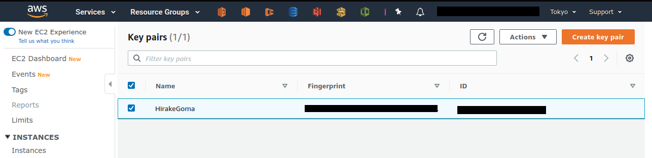
To do the same operation from the command line, use the following command:
$ aws ec2 delete-key-pair --key-name "OpenSesame"Lastly, delete the key from your local machine.
$ rm -f ~/.ssh/OpenSesame.pemNow, we’re all done cleaning up the cloud.
|
If you frequently start EC2 instances, you do not need to delete the SSH key every time. |
4.5. Summary
This is the end of the first part of the book. We hope you have been able to follow the contents without much trouble.
In Section 2, the definition of cloud and important terminology were explained, and then the reasons for using cloud were discussed. Then, in Section 3, AWS was introduced as a platform to learn about cloud computing, and the minimum knowledge and terminology required to use AWS were explained. In the hands-on session in Section 4, we used AWS CLI and AWS CDK to set up our own private server on AWS.
You can now experience how easy it is to start up and remove virtual servers (with just a few commands!). We mentioned in Section 2 that the most important aspect of the cloud is the ability to dynamically expand and shrink computational resources. We hope that the meaning of this phrase has become clearer through the hands-on experience. Using this simple tutorial as a template, you can customize the code for your own appplications, such as creating a virtual server to host your web pages, prepare an EC2 instance with a large number of cores to run scientific computations, and many more.
In the next chapter, you will experience solving more realistic problems based on the cloud technology you have learned. Stay tuned!
5. Scientific computing and machine learning in the cloud
In the modern age of computing, computational simulation and big data analysis are the major driving force of scientific and engineering research. The cloud is the best place to perform these large-scale computations. In Part II, which starts with this section, you will experience how to run scientific computation on the cloud through several hands-on experiences. As a specific subject of scientific computing, here we will focus on machine learning (deep learning).
In this book, we will use the PyTorch library to implement deep learning algorithms, but no knowledge of deep learning or PyTorch is required. The lecture focuses on why and how to run deep learning in the cloud, so we will not go into the details of the deep learning algorithm itself. Interested readers are refered to other books for the theory and implementation of deep neural network (column below).
5.1. Why use the cloud for machine learning?
The third AI boom started around 2010, and consequently machine learning is attracting a lot of attention not only in academic research but also in social and business contexts. In particular, algorithms based on multi-layered neural networks, known as deep learning, have revolutionized image recognition and natural language processing by achieving remarkably higher performance than previous algorithms.
The core feature of deep learning is its large number of parameters. As the layers become deeper, the number of weight parameters connecting the neurons between the layers increases. For example, the latest language model, GPT-3, contains as many as 175 billion parameters. With such a vast number of parameters, deep learning can achieve high expressive power and generalization performance.
Not only GPT-3, but also recent neural networks that achieve SOTA (State-of-the-Art) performance frequently contain parameters in the order of millions or billions. Naturally, training such a huge neural network is computationally expensive. As a result, it is not uncommon to see cases where the training takes more than a full day with a single workstation. With the rapid development of deep learning, the key to maximize research and business productivity is how to optimize the neural network with high throughput. The cloud is a very effective means to solve such problems! As we have seen in Section 4, the cloud can be used to dynamically launch a large number of instances, and execute computations in parallel. In addition, there are specially designed chips (e.g. GPUs) optimized for deep learning operations to accelerate the computation. By using the cloud, you gain access to inexhaustible supply of such specialized computing chips. In fact, it was reported that the training of GPT-3 was performed using Microsoft’s cloud, although the details have not been disclosed.
|
The details of the computational resources used in GPT-3 project are not disclosed in the paper, but there is an interesting discussion at Lambda’s blog (Lambda is a cloud service specializing in machine learning). According to the article, it would take 342 years and $4.6 million in cloud fees to train 175 billion parameters if a single GPU (NVIDIA V100) was used. The GPT-3 team was able to complete the training in a realistic amount of time by distributing the processing across multiple GPUs, but it is clear that this level of modeling can only be achieved by pushing the limits of cloud technology. |
5.2. Accelerating deep learning by GPU
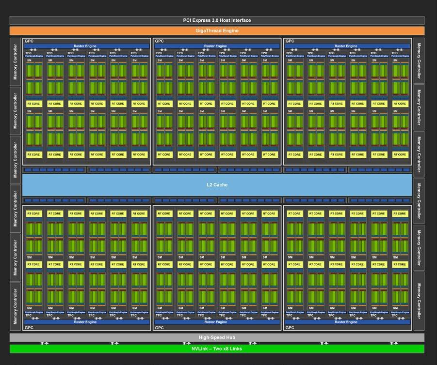
Here we will briefly talk about Graphics Processing Unit or GPU, which serves as an indispensable technology for deep learning.
As the name suggests, a GPU is originally a dedicated computing chip for producing computer graphics. In contrast to a CPU (Central Processing Unit) which is capable of general computation, a GPU is designed specifically for graphics operations. It can be found in familiar game consoles such as XBox and PS5, as well as in high-end notebook and desktop computers. In computer graphics, millions of pixels arranged on a screen need to be updated at video rates (30 fps) or higher. To handle this task, a single GPU chip contain hundreds to thousands of cores, each with relatively small computing power (Figure 17), and processes the pixels on the screen in parallel to achieve real-time rendering.
Although GPUs were originally developed for the purpose of computer graphics, since around 2010, some advanced programmers and engineers started to use GPU’s high parallel computing power for calculations other than graphics, such as scientific computations. This idea is called General-purpose computing on GPU or GPGPU. Due to its chip design, GPGPU is suitable for simple and regular operations such as matrix operations, and can achieve much higher speed than CPUs. Currently, GPGPU is employed in many fields such as molecular dynamics, weather simulation, and machine learning.
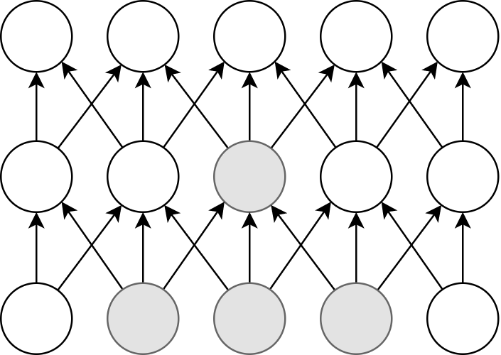
The operation that occurs most frequently in deep learning is the convolution operation, which transfers the output of neurons to the neurons in the next layer (Figure 18). Convolution is exactly the kind of operations that GPUs are good at, and by using GPUs instead of CPUs, learning can be dramatically accelerated, up to several hundred times.
Thus, GPUs are indispensable for machine learning calculations. However, they are quite expensive. For example, NVIDIA’s Tesla V100 chip, designed specifically for scientific computing and machine learning, is priced at about one million yen (ten thousand dollars). One million yen is quite a large investment just to start a machine learning project. The good news is, if you use the cloud, you can use GPUs with zero initial cost!
To use GPUs in AWS, you need to select an EC2 instance type equipped with GPUs, such as P2, P3, G3, and G4 instance family.
Table 3 lists representative GPU-equipped instance types as of this writing.
| Instance | GPUs | GPU model | GPU Mem (GiB) | vCPU | Mem (GiB) | Price per hour ($) |
|---|---|---|---|---|---|---|
p3.2xlarge |
1 |
NVIDIA V100 |
16 |
8 |
61 |
3.06 |
p3n.16xlarge |
8 |
NVIDIA V100 |
128 |
64 |
488 |
24.48 |
p2.xlarge |
1 |
NVIDIA K80 |
12 |
4 |
61 |
0.9 |
g4dn.xlarge |
1 |
NVIDIA T4 |
16 |
4 |
16 |
0.526 |
As you can see from Table 3, the price of GPU instances is higher than the CPU-only instances. Also note that older generation GPUs (K80 compared to V100) are offered at a lower price. The number of GPUs per instance can be selected from one to a maximum of eight.
The cheapest GPU instance type is g4dn.xlarge, which is equipped with a low-cost and energy-efficient NVIDIA T4 chip.
In the hands-on session in the later chapters, we will use this instance to perform deep learning calculations.
|
The prices in Table 3 are for |
|
The cost for |
6. Hands-on #2: Running Deep Learning on AWS
6.1. Preparation
In the second hands-on session, we will launch an EC2 instance equipped with a GPU and practice training and inference of a deep learning model.
The source code for the hands-on is available on GitHub at handson/mnist.
To run this hands-on, it is assumed that the preparations described in the first hands-on (Section 4.1) have been completed. There are no other preparations required.
|
In the initial state of your AWS account, the launch limit for G-type instances may be set to 0.
To check this, open the EC2 dashbord from the AWS console, and select If it is set to 0, you need to send a request to increase the limit via the request form. For details, see official documentation "Amazon EC2 service quotas". |
|
This hands-on uses a |
6.2. Reading the application source code
Figure 19 shows an overview of the application we will be deploying in this hands-on.
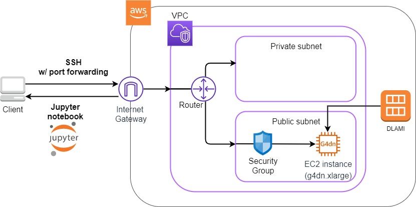
You will notice that many parts of the figure are the same as the application we created in the first hands-on session (Figure 10). With a few changes, we can easily build an environment to run deep learning! The three main changes are as follows.
-
Use a
g4dn.xlargeinstance type equipped with a GPU. -
Use a DLAMI (see below) with the programs for deep learning pre-installed.
-
Connect to the server using SSH with port forwarding option, and write and execute codes using Jupyter Notebook (see below) running on the server.
Let’s have a look at the source code (handson/mnist/app.py). The code is almost the same as in the first hands-on. We will explain only the parts where changes were made.
 1
 2
 3
 4
 5
 6
 7
 8
 9
10
11
12
13
14
15
16
17
18
19
20
21
22
23
24
25
26
27
28
29
30
31
32
33
34
35
36
37
38
39
40
class Ec2ForDl(Stack):

    def __init__(self, scope: Construct, construct_id: str, key_name: str, **kwargs) -> None:
        super().__init__(scope, construct_id, **kwargs)

        vpc = ec2.Vpc(
            self, "Ec2ForDl-Vpc",
            max_azs=1,
            ip_addresses=ec2.IpAddresses.cidr("10.10.0.0/23"),
            subnet_configuration=[
                ec2.SubnetConfiguration(
                    name="public",
                    subnet_type=ec2.SubnetType.PUBLIC,
                )
            ],
            nat_gateways=0,
        )

        sg = ec2.SecurityGroup(
            self, "Ec2ForDl-Sg",
            vpc=vpc,
            allow_all_outbound=True,
        )
        sg.add_ingress_rule(
            peer=ec2.Peer.any_ipv4(),
            connection=ec2.Port.tcp(22),
        )

        host = ec2.Instance(
            self, "Ec2ForDl-Instance",
            instance_type=ec2.InstanceType("g4dn.xlarge"), (1)
            machine_image=ec2.MachineImage.generic_linux({
                "us-east-1": "ami-060f07284bb6f9faf",
                "ap-northeast-1": "ami-09c0c16fc46a29ed9"
            }), (2)
            vpc=vpc,
            vpc_subnets=ec2.SubnetSelection(subnet_type=ec2.SubnetType.PUBLIC),
            security_group=sg,
            key_name=key_name
        )
| 1 | Here, we have selected the g4dn.xlarge instance type (in the first hands-on, it was t2.micro).
As already mentioned in Section 5, the g4dn.xlarge is an instance with a low-cost model GPU called NVIDIA T4.
It has 4 CPU cores and 16GB of main memory. |
| 2 | Here, we are using
Deep Learning Amazon Machine Image; DLAMI,
an AMI with varisous programs for deep learning pre-installed.
Note that in the first hands-on, we used an AMI called Amazon Linux.
The ID of the AMI must be specified for each region, and here we are supplying IDs for us-east-1 and ap-northeast-1. |
|
In the code above, the AMI IDs are only defined in |
6.2.1. DLAMI (Deep Learning Amazon Machine Image)
AMI (Amazon Machine Image) is a concept that roughly corresponds to an OS (Operating System). Naturally, a computer cannot do anything without an OS, so it is necessary to "install" some kind of OS whenever you start an EC2 instance. The equivalent of the OS that is loaded in EC2 instance is the AMI. For example, you can choose Ubuntu AMI to launch your EC2 instance. As alternative options, you can select Windows Server AMI or Amazon Linux AMI, which is optimized for use with EC2.
However, it is an oversimplification to understand AMI as just an OS. AMI can be the base (empty) OS, but AMI can also be an OS with custom programs already installed. If you can find an AMI that has the necessary programs installed, you can save a lot of time and effort in installing and configuring the environment yourself. To give a concrete example, in the first hands-on session, we showed an example of installing Python 3.6 on an EC2 instance, but doing such an operation every time the instance is launched is tedious!
In addition to the official AWS AMIs, there are also AMIs provided by third parties. It is also possible to create and register your own AMI (see official documentation). You can search for AMIs from the EC2 dashboard. Alternatively, you can use the AWS CLI to obtain a list with the following command (also see official documentation).
$ aws ec2 describe-images --owners amazonDLAMI (Deep Learning AMI)
is an AMI pre-packaged with deep learning tools and programs.
DLAMI comes with popular deep learning frameworks and libraries such as TensorFlow and PyTorch, so you can run deep learning applications immediately after launching an EC2 instance.
In this hands-on, we will use a DLAMI based on Amazon Linux 2 (AMI ID = ami-09c0c16fc46a29ed9). Let’s use the AWS CLI to get the details of this AMI.
$ aws ec2 describe-images --owners amazon --image-ids "ami-09c0c16fc46a29ed9"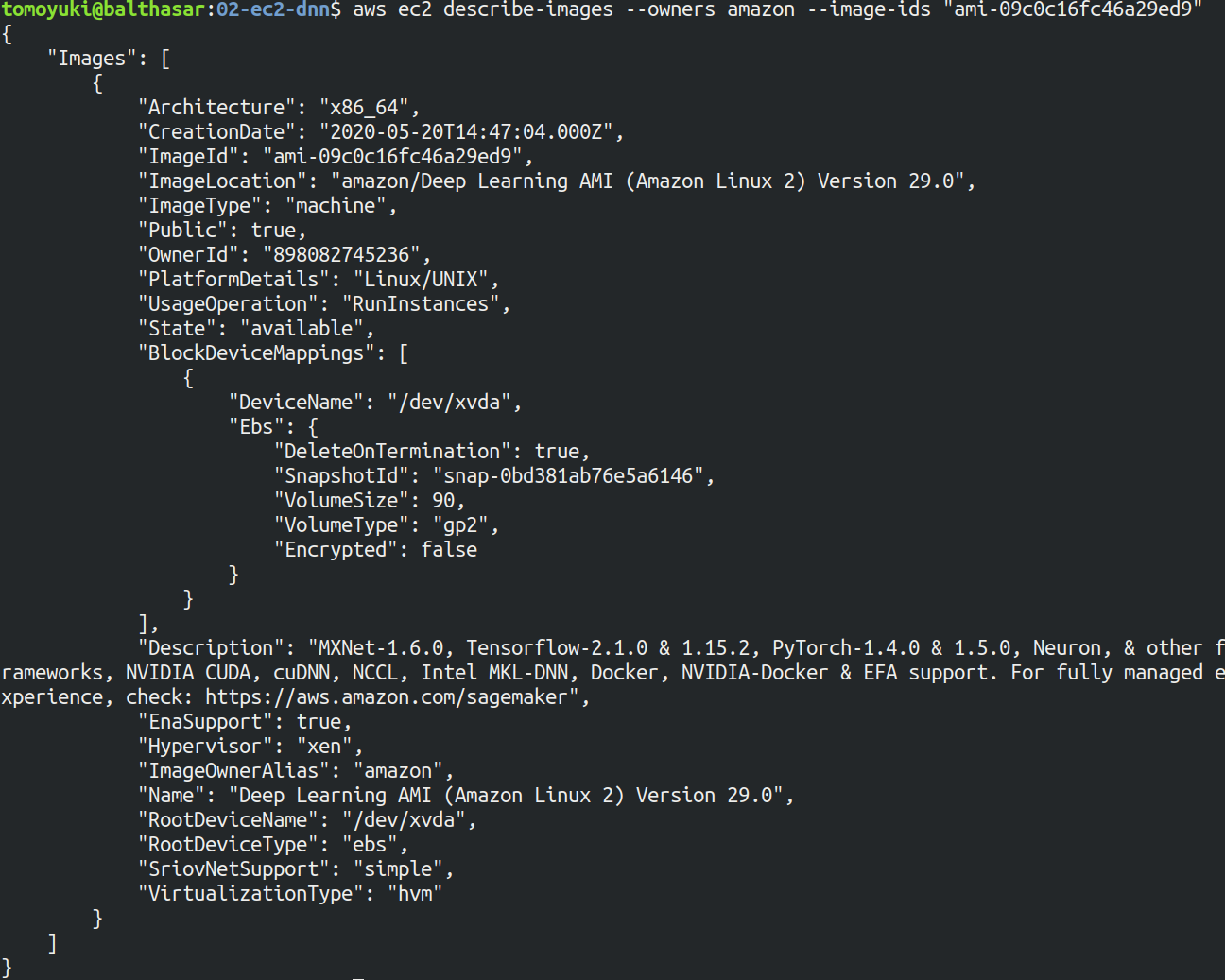
You should get an output like Figure 20. From the output, we can see that the DLAMI has PyTorch versions 1.4.0 and 1.5.0 installed.
|
What exactly is installed in DLAMI? For the interested readers, here is a brief explanation (Reference: official documentation "What Is the AWS Deep Learning AMI?"). At the lowest level, the GPU driver is installed. Without the GPU driver, the OS cannot exchange commands with the GPU. The next layer is CUDA and cuDNN. CUDA is a language developed by NVIDIA for general-purpose computing on GPUs, and has a syntax that extends the C++ language. cuDNN is a deep learning library written in CUDA, which implements operations such as n-dimensional convolution. This is the content of the "Base" DLAMI. The "Conda" DLAMI has libraries such as |
6.3. Deploying the application
Now that we understand the application source code, let’s deploy it.
The deployment procedure is almost the same as the first hands-on.
Here, only the commands are listed (lines starting with # are comments).
If you have forgotten the meaning of each command, review the first hands-on.
You should not forget to set the access key (Section 14.3).
# move to the project directory
$ cd handson/mnist

# create venv and install dependent libraries
$ python3 -m venv .env
$ source .env/bin/activate
$ pip install -r requirements.txt

# Generate SSH key
$ export KEY_NAME="OpenSesame"
$ aws ec2 create-key-pair --key-name ${KEY_NAME} --query 'KeyMaterial' --output text > ${KEY_NAME}.pem
$ mv OpenSesame.pem ~/.ssh/
$ chmod 400 ~/.ssh/OpenSesame.pem

# Deploy!
$ cdk deploy -c key_name="OpenSesame"|
If you did not delete the SSH key you created in the first hands-on, you do not need to create another SSH key. Conversely, if an SSH with the same name already exists, the key generation command will output an error. |
If the deployment is executed successfully, you should get an output like Figure 21.
Note the IP address of your instance (the string following InstancePublicIp).
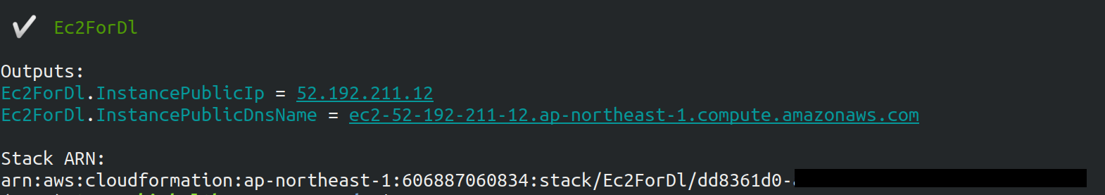
cdk deploy6.4. Log in to the instance
Let’s log in to the deployed instance using SSH.
To connect to Jupyter Notebook, which we will be using later, we must log in with the port forwarding option (-L).
$ ssh -i ~/.ssh/OpenSesame.pem -L localhost:8931:localhost:8888 ec2-user@<IP address>Port forwarding means that the connection to a specific address on the client machine is forwarded to a specific address on the remote machine via SSH encrypted communication.
The option -L localhost:8931:localhost:8888 means to forward the access to localhost:8931 of your local machine to the address of localhost:8888 of the remote server
(The number following : specifies the TCP/IP port number).
On port 8888 of the remote server, Jupyter Notebook (described below) is running.
Therefore, you can access Jupyter Notebook on the remote server by accessing localhost:8931 on the local machine (Figure 22).
This type of SSH connection is called a tunnel connection.
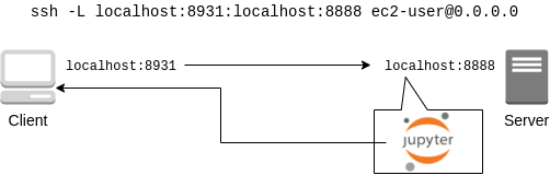
|
In the port forwarding options, the port number ( Jupyter Notebook uses port 8888 by default. Therefore, it is recommended to use port 8888 for the remote side. |
|
Don’t forget to assign the IP address of your instance to the |
|
For those who have done deployment using Docker: SSH login must be done from outside of Docker. This is because the web browser that opens Jupyter is outside of Docker. |
After logging in via SSH, let’s check the status of the GPU. Run the following command.
$ nvidia-smiYou should get output like Figure 23. The output shows that one Tesla T4 GPU is installed. Other information such as the GPU driver, CUDA version, GPU load, and memory usage can be checked.
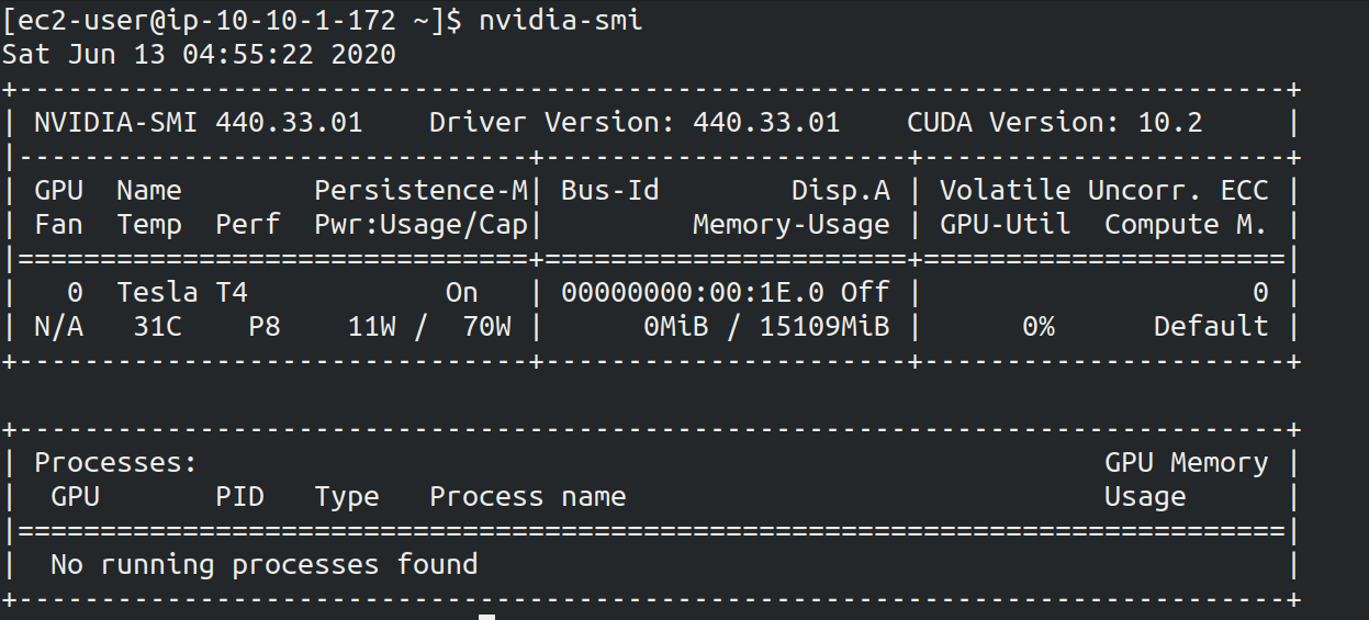
nvidia-smi6.5. Launching Jupyter Notebook
Jupyter Notebook is a tool for writing and running Python programs interactively. Jupyter is accessed via a web browser, and can display plots and table data beautifully as if you were writing a notebook (Figure 24). If you are familiar with Python, you have probably used it at least once.
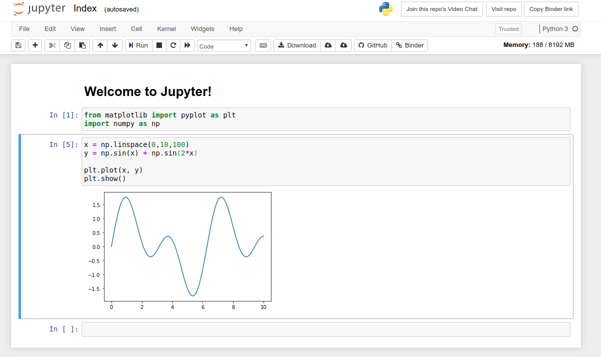
In this hands-on session, we will run a deep learning program interactively using Jupyter Notebook. Jupyter is already installed on DLAMI, so you can start using it without any configuration.
Now, let’s start Jupyter Notebook server. On the EC2 instance where you logged in via SSH, run the following command.
$ cd ~ # go to home directory
$ jupyter notebook
When you run this command, you will see output like Figure 25.
From this output, we can see that the Jupyter server is launched at the address localhost:8888 of the EC2 instance.
The string ?token=XXXX following localhost:8888 is a temporary token used for accessing Jupyter.
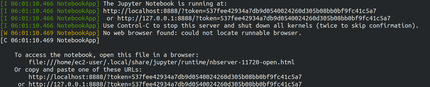
|
When you start Jupyter Notebook for the first time, it may take a few minutes to start up. Other operations are also slow immediately after startup, but after running a few commands, the system becomes agile and responsive. This phenomenon is thought to be caused by the way the AWS operates the virtual machines with GPUs. |
Since the port forwarding option was added to the SSH connection, you can access localhost:8888, where Jupyter is running, from localhost:8931 on your local machine.
Therefore, to access Jupyter from the local machine, you can access the following address from a web browser (Chrome, FireFox, etc.).
http://localhost:8931/?token=XXXXRemember to replace ?token=XXXX with the actual token that was issued when Jupyter server was started above.
If you access the above address, the Jupyter home screen should be loaded (Figure 26). Now, Jupyter is ready!
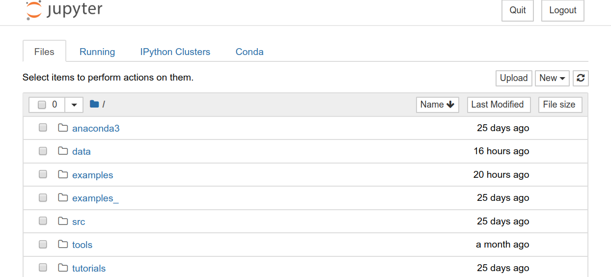
|
Minimalistic guide to Jupyter Notebook
For a list of shortcuts, see the blog by Ventsislav Yordanov. |
6.6. Introduction to PyTorch
PyTorch is an open source deep learning library that is being developed by the Facebook AI Research LAB (FAIR). PyTorch is one of the most popular deep learning libraries at the time of writing, and is being used by Tesla in their self-driving project, to name a few. In this hands-on session, we will use PyTorch to practice deep learning.
|
A Brief History of PyTorch In addition to PyTorch, Facebook has been developing a deep learning framework called Caffe2 (The original Caffe was created by Yangqing Jia, a PhD student at UC Berkley). Caffe2 was merged into the PyTorch project in 2018. In December 2019, it was also announced that Chainer, which was developed by Preferred Networks in Japan, will also end its development and collaborate with the PyTorch development team. (For more information, see press release). PyTorch has a number of APIs that were inspired by Chainer even before the integration, and the DNA of Chainer is still being carried over to PyTorch…! |
Before we move on to some serious deep learning calculations, let’s use the PyTorch library to get a feel for what it is like to run computations on the GPU.
First, we’ll create a new notebook. Click "New" in the upper right corner of the Jupyter home screen, select the environment "conda_pytorch_p36", and create a new notebook (Figure 27). In the "conda_pytorch_p36" virtual environment, PyTorch is already installed.
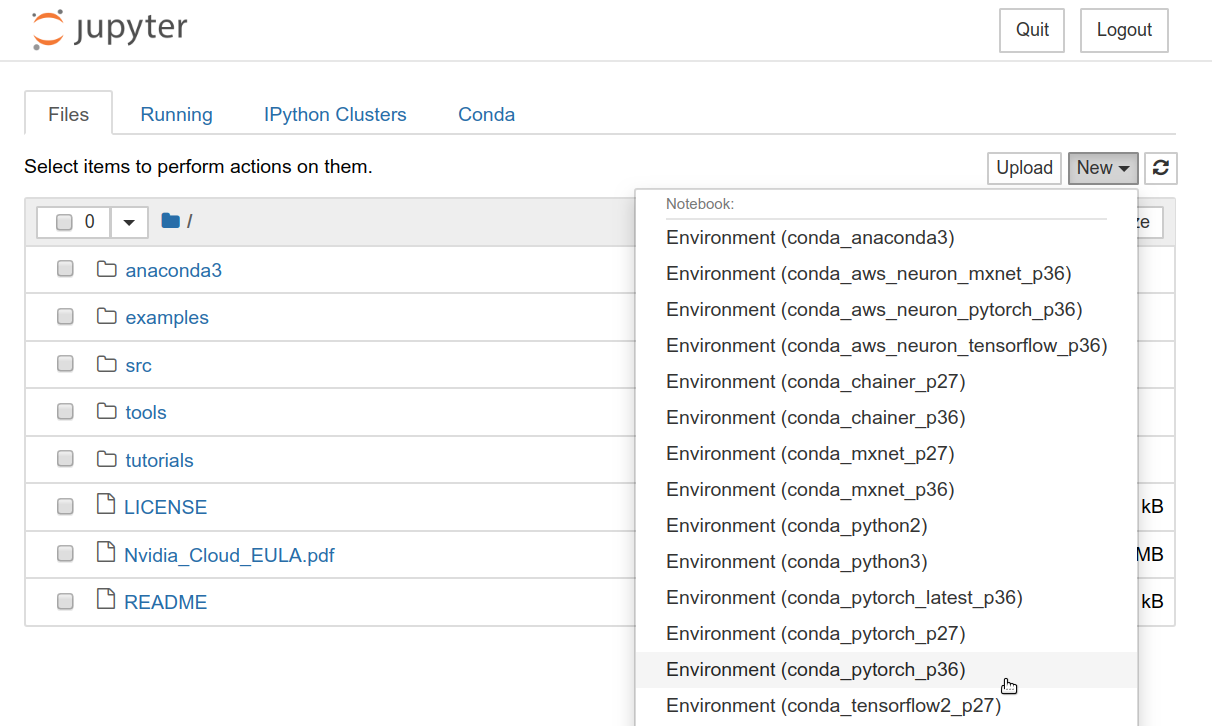
Here, we will write and execute the following program (Figure 28).
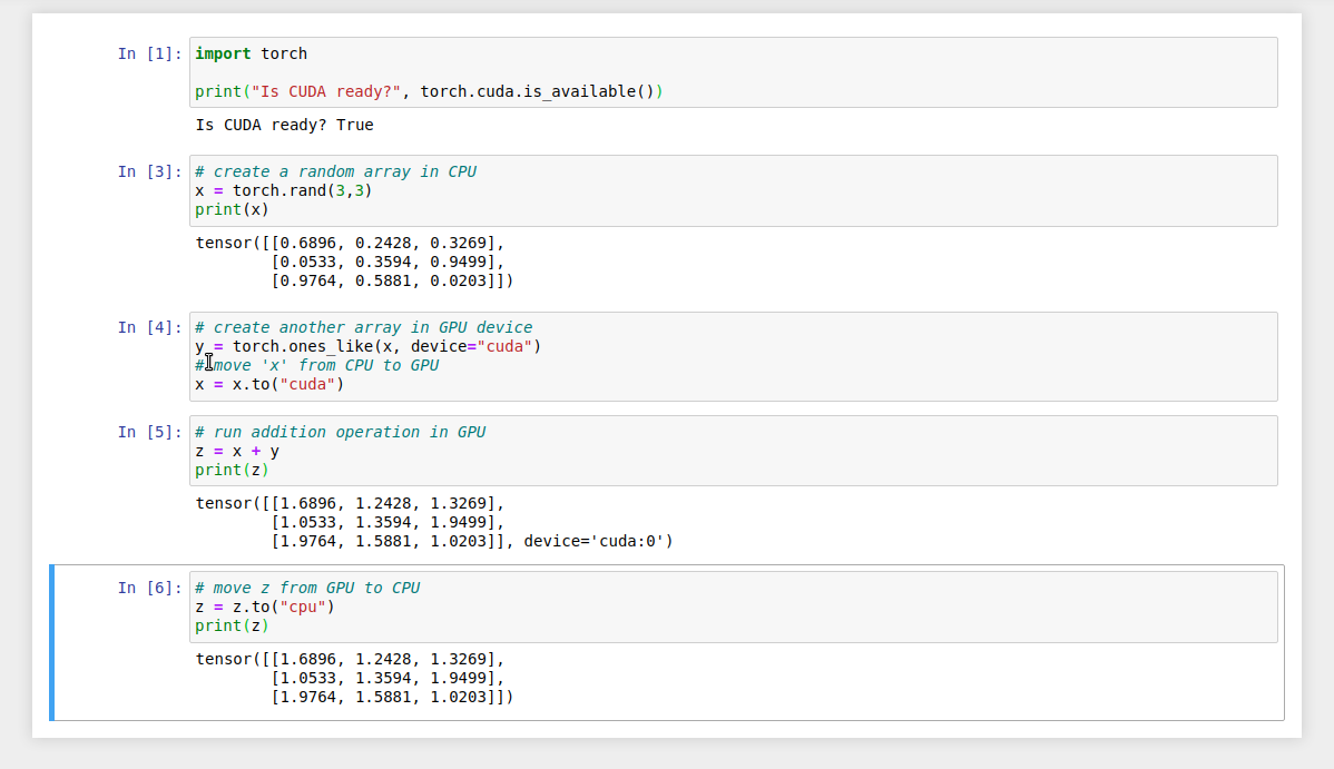
First, we import PyTorch. In addition, we check that the GPU is available.
1
2
import torch
print("Is CUDA ready?", torch.cuda.is_available())
Output:
Is CUDA ready? TrueNext, let’s create a random 3x3 matrix x on CPU.
1
2
x = torch.rand(3,3)
print(x)
Output:
tensor([[0.6896, 0.2428, 0.3269],
        [0.0533, 0.3594, 0.9499],
        [0.9764, 0.5881, 0.0203]])
Next, we create another matrix y on GPU.
We also move the matrix x on GPU.
1
2
y = torch.ones_like(x, device="cuda")
x = x.to("cuda")
Then, we perform the addition of the matrix x and y on GPU.
1
2
z = x + y
print(z)
Output:
tensor([[1.6896, 1.2428, 1.3269],
        [1.0533, 1.3594, 1.9499],
        [1.9764, 1.5881, 1.0203]], device='cuda:0')
Lastly, we bring the matrix on GPU back on CPU.
1
2
z = z.to("cpu")
print(z)
Output:
tensor([[1.6896, 1.2428, 1.3269],
        [1.0533, 1.3594, 1.9499],
        [1.9764, 1.5881, 1.0203]])
The above examples are just the rudiments of GPU-based computation, but we hope you get the idea. The key is to explicitly exchange data between the CPU and GPU. This example demonstrated an operation on 3x3 matrix, so the benefit of using GPU is almost negligible. However, when the size of the matrix is in the thousands or tens of thousands, the GPU becomes much more powerful.
|
The finished Jupyter Notebook is available at /handson/mnist/pytorch/ pytorch_get_started.ipynb. You can upload this file by clicking "Upload" in the upper right corner of the Jupyter window, and run the code. However, it is more effective to write all the code by yourself when you study. That way the code and concepts will stick in your memory better. |
Let’s benchmark the speed of the GPU and the CPU and compare the performance. We will use Jupyter’s %time magic command to measure the execution time.
First, using the CPU, let’s measure the speed of computing the matrix product of a 10000x10000 matrix. Continuing from the notebook we were just workin with, paste the following code and run it.
1
2
3
4
5
6
s = 10000
device = "cpu"
x = torch.rand(s, s, device=device, dtype=torch.float32)
y = torch.rand(s, s, device=device, dtype=torch.float32)

%time z = torch.matmul(x,y)
The output should look something like shown below. This means that it took 5.8 seconds to compute the matrix product (note that the measured time varies with each run).
CPU times: user 11.5 s, sys: 140 ms, total: 11.6 s
Wall time: 5.8 s
Next, let’s measure the speed of the same operation performed on the GPU.
1
2
3
4
5
6
7
s = 10000
device = "cuda"
x = torch.rand(s, s, device=device, dtype=torch.float32)
y = torch.rand(s, s, device=device, dtype=torch.float32)
torch.cuda.synchronize()

%time z = torch.matmul(x,y); torch.cuda.synchronize()
The output should look something like shown below. This time, the computation was completed in 553 milliseconds!
CPU times: user 334 ms, sys: 220 ms, total: 554 ms
Wall time: 553 ms|
In PyTorch, operations on the GPU are performed asynchronously.
For this reason, the benchmark code above embeds the statement |
From this benchmark, we were able to observe about 10 times speedup by using the GPU. The speed-up performance depends on the type of operation and the size of the matrix. The matrix product is one of the operations where the speedup is expected to be highest.
6.7. MNIST Handwritten Digit Recognition Task
Now that we have covered the concepts and prerequisites for deep learning computations on AWS, it’s time to run a real deep learning application.
In this section, we will deal with one of the most elementary and famous machine learning tasks, handwritten digit recognition using the MNIST dataset (Figure 29). This is a simple task where we are given images of handwritten numbers from 0 to 9 and try to guess what the numbers are.
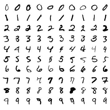
Here, we will use Convolutional Neural Network (CNN) to solve the MNIST task.
The source code is available on GitHub at
/handson/minist/pytorch/.
The relevant files are mnist.ipynb and simple_mnist.py in this directory.
This program is based on
PyTorch’s official example project collection,
with some modifications.
First, let’s upload simple_mnist.py, which contains custom classes and functions (Figure 30).
Go to the home of the Jupyter, click on the "Upload" button in the upper right corner of the screen, and select the file to upload.
Inside this Python program, we defined the CNN model and the parameter optimization method.
We won’t explain the contents of the program, but readers interested in the subject can read the source code and learn for themselves.
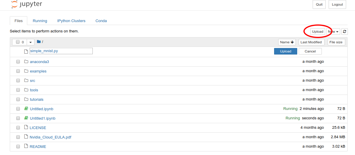
simple_mnist.pyOnce you have uploaded simple_mnist.py, you can create a new notebook.
Be sure to select the "conda_pytorch_p36" environment.
Once the new notebook is up and running, let’s import the necessary libraries first.
1
2
3
4
5
6
7
8
import torch
import torch.optim as optim
import torchvision
from torchvision import datasets, transforms
from matplotlib import pyplot as plt

# custom functions and classes
from simple_mnist import Model, train, evaluate
The
torchvision
package contains some useful functions, such as loading MNIST datasets.
The above code also imports custom classes and functions (Model, train, evaluate) from simple_mnist.py that we will use later.
Next, we download the MNIST dataset. At the same time, we are normalizing the intensity of the images.
1
2
3
4
5
6
7
8
transf = transforms.Compose([transforms.ToTensor(),
                             transforms.Normalize((0.1307,), (0.3081,))])

trainset = datasets.MNIST(root='./data', train=True, download=True, transform=transf)
trainloader = torch.utils.data.DataLoader(trainset, batch_size=64, shuffle=True)

testset = datasets.MNIST(root='./data', train=False, download=True, transform=transf)
testloader = torch.utils.data.DataLoader(testset, batch_size=1000, shuffle=True)
The MNIST dataset consists of 28x28 pixel monochrome square images and corresponding labels (numbers 0-9). Let’s extract some of the data and visualize them. You should get an output like Figure 31.
 1
 2
 3
 4
 5
 6
 7
 8
 9
10
11
12
13
14
examples = iter(testloader)
example_data, example_targets = examples.next()

print("Example data size:", example_data.shape)

fig = plt.figure(figsize=(10,4))
for i in range(10):
    plt.subplot(2,5,i+1)
    plt.tight_layout()
    plt.imshow(example_data[i][0], cmap='gray', interpolation='none')
    plt.title("Ground Truth: {}".format(example_targets[i]))
    plt.xticks([])
    plt.yticks([])
plt.show()
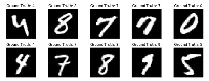
Next, we define the CNN model.
1
2
model = Model()
model.to("cuda") # load to GPU
The Model class is defined in simple_mnist.py.
We will use a network with two convolutional layers and two fully connected layers, as shown in Figure 32.
The output layer is the Softmax function, and the loss function is the negative log likelihood function (NLL).
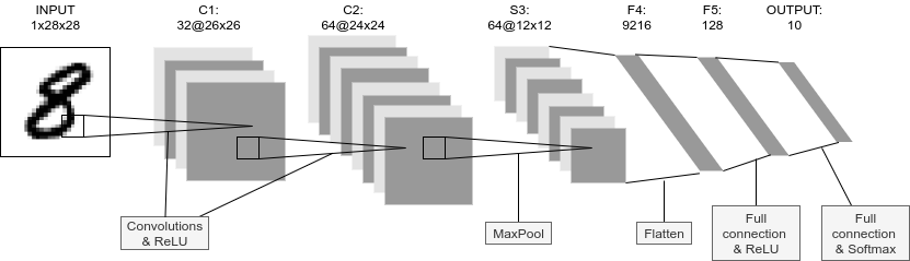
Next, we define an optimization algorithm to update the parameters of the CNN. We use the Stochastic Gradient Descent (SGD) method.
1
optimizer = optim.SGD(model.parameters(), lr=0.01, momentum=0.5)
Now, we are ready to go. Let’s start the CNN training loop!
 1
 2
 3
 4
 5
 6
 7
 8
 9
10
11
12
train_losses = []
for epoch in range(5):
    losses = train(model, trainloader, optimizer, epoch)
    train_losses = train_losses + losses
    test_loss, test_accuracy = evaluate(model, testloader)
    print(f"\nTest set: Average loss: {test_loss:.4f}, Accuracy: {test_accuracy:.1f}%\n")

plt.figure(figsize=(7,5))
plt.plot(train_losses)
plt.xlabel("Iterations")
plt.ylabel("Train loss")
plt.show()
In this example, we are training for 5 epochs. Using a GPU, computation like this can be completed in about a minute.
The output should be a plot similar to Figure 33. You can see that the value of the loss function is decreasing (i.e. the accuracy is improving) as the iteration proceeds.
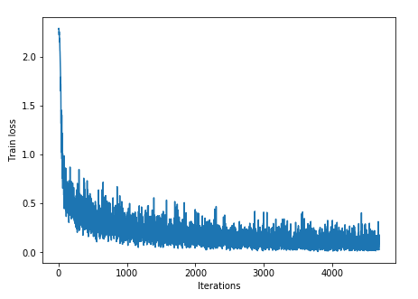
Let’s visualize the inference results of the learned CNN. By running the following code, you should get an output like Figure 34. If you closely look at this figure, the second one from the right in the bottom row looks almost like a "1", but it is correctly inferred as a "9". It looks like we have managed to create a pretty smart CNN!
 1
 2
 3
 4
 5
 6
 7
 8
 9
10
11
12
13
14
model.eval()

with torch.no_grad():
    output = model(example_data.to("cuda"))

fig = plt.figure(figsize=(10,4))
for i in range(10):
    plt.subplot(2,5,i+1)
    plt.tight_layout()
    plt.imshow(example_data[i][0], cmap='gray', interpolation='none')
    plt.title("Prediction: {}".format(output.data.max(1, keepdim=True)[1][i].item()))
    plt.xticks([])
    plt.yticks([])
plt.show()
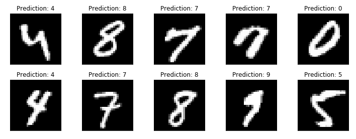
Finally, we save the parameters of the trained neural network as a file named mnist_cnn.pt.
This way, you can reproduce the learned model and use it for another experiment anytime in the future.
1
torch.save(model.state_dict(), "mnist_cnn.pt")
That’s it! We have experienced all the steps to set up a virtual server in the AWS cloud and perform the deep learning computation. Using the GPU instance in the cloud, we were able to train a neural network to solve the MNIST digit recognition task. Interested readers can use this hands-on as a template to run their own deep learning applications.
6.8. Deleting the stack
Now we are done with the GPU instance. Before the EC2 cost builds up, we should delete the instance we no longer use.
As in the first hands-on session, we can delete the instance using the AWS CloudFormation console, or using the AWS CLI (see Section 4.4.8).
$ cdk destroy|
Make sure you delete your stack after the exercise!
If you do not do so, you will continue to be charged for the EC2 instance!
|
7. Introduction to Docker
In the hands-on exercises described in the previous chapters, we have set up a single server, logged in to it via SSH, and performed calculations by typing commands. In other words, we have been using the cloud as an extension of our personal computers. This kind of use of the cloud as a personal computer is, of course, convenient and has many potential applications. However, the true value of the cloud is not fully demonstrated by this alone. As described in Section 2, the greatest strength of the modern cloud is the ability to freely expand the scale of computing. That is to say, the true potential of the cloud can only be demonstrated by processing large amounts of data by running many servers simultaneously and executing multiple jobs in a distributed parallel fashion.
Using the three sections starting from this chapter (Section 7, Section 8, Section 9), we would like to show you a glimpse of how to build a large-scale computing system using the cloud to tackle challenges like the big data analysis. In particular, we would like to focus our discussion on how to apply the deep learning to big data. As a prelude to this, this chapter introduces a virtualization software called Docker. It would not be an exaggeration to say that modern cloud computing would not be possible without Docker. Docker is very useful not only for cloud computing, but also for local computation. This is a bit of a departure from AWS, but it’s important to understand Docker well enough to move forward.
7.1. Scaling up machine learning
We have been repeatedly calling for "large-scale computing systems," but what exactly does that mean? Let’s take machine learning as an example, and talk about a computer system for processing large data.
Suppose we want to train a deep learning model with a very large number of parameters, such as GPT-3 introduced in Section 5. If you want to perform such a computation, a single server will not have enough computing power. Therefore, the typical design of a computing system would be a model shown in Figure 35. Namely, a large amount of training data is distributed in small chunks across multiple machines, and the parameters of the neural network are optimized in parallel.
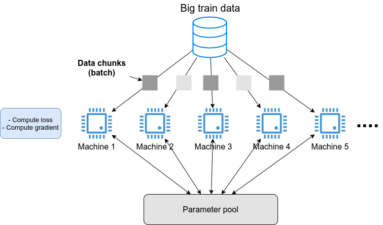
Or, let’s say you want to apply a trained model to a large amount of data for analysis. For example, you have a SNS platform and you are given a large number of images, and you want to label what is in each photo. In such a case, an architecture such as the one shown in Figure 36 can be considered, in which a large amount of data is divided among multiple machines, and each machine performs inference computation.
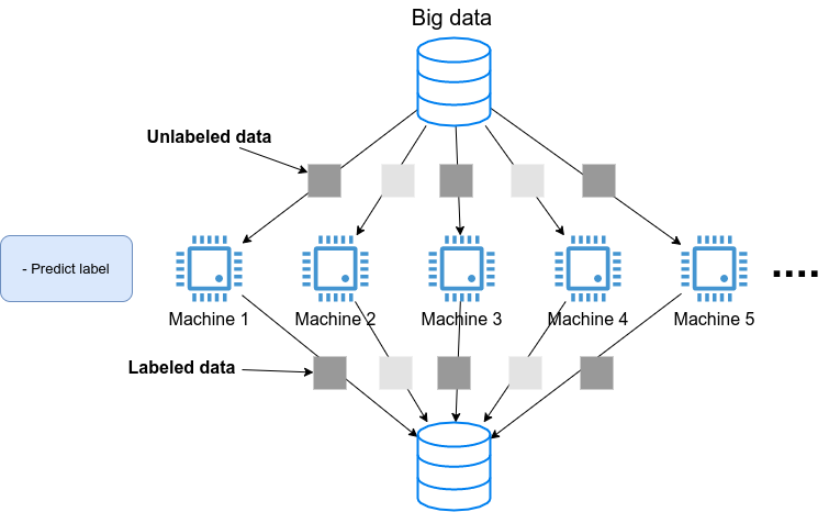
How can such applications that run multiple computers simultaneously be implemented in the cloud?
One important point is that the multiple machines running Figure 35 and Figure 36 have basically the same OS and computing environment. Here, it is possible to perform the same installation operations on each machine as one would do on an individual computer, but this would be very time-consuming and cumbersome to maintain. In other words, in order to build a large-scale computing system, it is necessary to have a mechanism that allows to easily replicate the computing environment.
To achieve this goal, a software called Docker is used.
7.2. What is Docker?
Docker is software for running a separate computing environment independent of the host OS in a virtual environment called a container. Docker makes it possible to package all programs, including the OS, in a compact package (a packaged computing environment is called an image). Docker makes it possible to instantly replicate a computing environment on a cloud server, and to create a system for running multiple computers simultaneously, as seen in Figure 36.
Docker was developed by Solomon Hykes and his fellows in 2013, and since then it has exploded in popularity, becoming core software not only for cloud computing but also in the context of machine learning and scientific computing. Docker is available free of charge, except for enterprise products, and its core is available as an open source project. Docker is available for Linux, Windows, and Mac operating systems. Conceptually, Docker is very similar to a virtual machine (VM). Comparing Docker with VM is a very useful way to understand what Docker is, so here we take this approach.
A virtual machine (VM) is a technology that allows to run virtualized operating systems on top of a host machine (Figure 38). A VM has a layer called a hypervisor. The hypervisor first divides the physical computing resources (CPU, RAM, network, etc.) and virtualizes them. For example, if the host machine has four physical CPU cores, the hypervisor can virtually divide them into (2,2) pairs. The OS running on the VM is allocated virtualized hardware by the hypervisor. OSes running on VM are completely independent. For example, OS-A cannot access the CPU or memory space allocated to OS-B (this is called isolation). Famous software for creating VMs includes VMware, VirtualBox, and Xen. EC2, which we have used earlier, basically uses VM technology to present the user with a virtual machine with the desired specifications.
Docker, like VM, is a technology for running a virtualized OS on a host OS. In contrast to VMs, Docker does not rely on hardware-level virtualization; all virtualization is done at the software level (Figure 38). The virtual OS running on Docker relies on the host OS for much of its functionality, and as a result is very compact. Consequently, the time required to boot a virtual OS with Docker is much faster than with a VM. It is also important to note that the size of the packaged environment (i.e., image) is much smaller than that of a full OS, which greatly speeds up communication over the network. In addition, some implementations of VMs are known to have lower performance than metal (metal means OS running directly on physical hardware) due to the overhead at the hypervisor layer. Docker is designed to be able to achieve almost the same performance as metal.
There are many other differences between Docker and VM, but we will not go into details here. The important point is that Docker is a tool for creating a very compact and high-performance virtual computing environment. Because of its ease of use and lightness, Docker has been adopted in many cloud systems since its introduction in 2013, and it has become an essential core technology in the modern cloud.
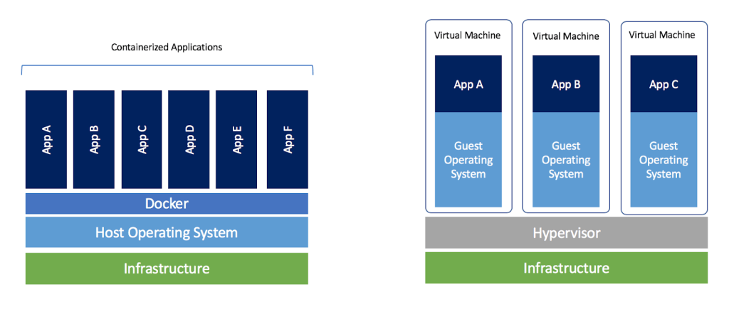
7.3. Docker tutorial
The most effective way to understand what Docker is is to actually try it out. In this section, I will give a brief tutorial on Docker.
For Docker installation, please refer to Section 14.6 and official documentation. The following assumes that you have already installed Docker.
7.3.1. Docker terminology
To get you started with Docker, let us first define some key terms.
Figure 39 shows the general steps to start Docker. A packaged computing environment is called an image. Images can be downloaded from repositories such as Docker Hub, or you can create your own custom images. The file that describes the "recipe" for creating an image is called Dockerfile. The operation to create an image from a Dockerfile is called build. When an image is loaded in to the host machine’s memory, the virtual environment is ready, which is called a container. The command used to start the container is run.
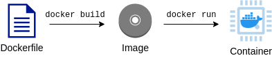
7.3.2. Downloading an image
The packaged Docker virtual environment (=image) can be downloaded from Docker Hub. Docker Hub hosts Docker images created by individuals, companies, and organizations, and is open to the public just like GitHub.
For example, Ubuntu images are available at
https://hub.docker.com/_/ubuntu [the official Ubuntu repository],
and can be downloaded to the local machine by using the pull command.
$ docker pull ubuntu:18.04Here, the string following the : (colon) in the image name is called a tag and is mainly used to specify the version.
|
The |
7.3.3. Launching a container
To launch a container from the image, use the run command.
$ docker run -it ubuntu:18.04Here, -it is an option required to start an interactive shell session.
When this command is executed, the virtualized Ubuntu will be launched and commands can be typed from the command line (Figure 40). A computational environment (runtime) in running state is called a container.

The ubuntu:18.04 image used here is an empty Ubuntu OS, but there are other images available with some programs already installed.
This is similar to the concept of DLAMI as we saw in Section 6.
For example, an image with PyTorch already installed is available at
PyTorch’s official Docker Hub repository.
Let’s launch this image.
$ docker run -it pytorch/pytorch
|
When you run |
Once the PyTorch container is up and running, lanch a Python shell and test importing pytorch.
$ python3
Python 3.7.7 (default, May  7 2020, 21:25:33)
[GCC 7.3.0] :: Anaconda, Inc. on linux
Type "help", "copyright", "credits" or "license" for more information.
>>> import torch
>>> torch.cuda.is_available()
False
As we saw in these examples, Docker makes it possible to easily reproduce a computing environment with a specific OS and program.
7.3.4. Making your own image
It is also possible to create your own image which includes any softwares your application may require.
For example, the docker image provided for the hands-on exercises in this book comes with Python, Node.js, AWS CLI, and AWS CDK already installed, so you can run the hands-on program immediately after pulling the image.
To create a custom docker image, all you need to do is to prepare a file named Dockerfile and describe what programs you want to install in it.
As an example, let’s take a look at the Docker image recipe provided in this book (docker/Dockerfile).
FROM node:12
LABEL maintainer="Tomoyuki Mano"

RUN apt-get update \
    && apt-get install nano

(1)
RUN cd /opt \
    && curl -q "https://www.python.org/ftp/python/3.7.6/Python-3.7.6.tgz" -o Python-3.7.6.tgz \
    && tar -xzf Python-3.7.6.tgz \
    && cd Python-3.7.6 \
    && ./configure --enable-optimizations \
    && make install

RUN cd /opt \
    && curl "https://awscli.amazonaws.com/awscli-exe-linux-x86_64.zip" -o "awscliv2.zip" \
    && unzip awscliv2.zip \
    && ./aws/install

(2)
RUN npm install -g aws-cdk@1.100

# clean up unnecessary files
RUN rm -rf /opt/*

# copy hands-on source code in /root/
COPY handson/ /root/handson
We won’t go into detail about Dockerfile.
But, for example, in the code above, <1> installs Python 3.7, and <2> installs the AWS CDK.
You can create your own Docker image by describing the installation commands one by one in the same way as you would do for a real OS.
Once the image is created, it can be distributed to others so that they can easily reproduce the same computing environment.
"That program runs in my computer…" is a common phrase among novice programmers. With Docker, you say goodbye to those concerns. In this sense, Docker’s usefulness and versatility is extremely high even in the contexts other than cloud computing.
7.4. Elastic Container Service (ECS)

As we have explained so far, Docker is a highly versatile and powerful tool to replicate and launch a virtual computing environment. As the last topic of this section, we will talk about how to build a computing system using Docker on AWS.
Elastic Container Service (ECS) is a tool for creating Docker-based compute clusters on AWS (Figure 41). Using ECS, you can define tasks using Docker images, create a compute cluster, and add or remove instances in the compute cluster.
Figure 42 shows an overview of ECS. The ECS accepts computation jobs managed in units called tasks. When a task is submitted to the system, ECS first downloads the Docker image specified by the task from an external registry. The external registry can be Docker Hub or AWS' own image registry, ECR (Elastic Container Registry).
The next important role of ECS is task placement. By selecting a virtual instance with low computational load in a predefined cluster, ECS places a Docker image on it, and the task is started. When we say "select a virtual instance with low computational load," the specific strategy and policy for this selection depends on the parameters specified by the user.
Scaling of clusters is another important role of ECS. Scaling refers to the operation of monitoring the computational load of the instances in a cluster, and starting and stopping the instances according to the total load on the cluster. When the computational load of the entire cluster exceeds a specified threshold (e.g., 80% utilization), a new virtual instance is launched (an operation called scale-out). When the computational load is below a certain threshold, unnecessary instances are stoped (an operation called scale-in). The scaling of a cluster is achieved by the ECS cooperating with other AWS services. Specifically, ECS is most commonly paired with Auto scaling group (ASG) or Fargate. ASG and Fargate, respectively will be covered in Section 9 and Section 8.
ECS automatically manages the above explained operations for you. Once the parameters for cluster scaling and task placement are specified, the user can submit a large number of tasks, almost without thinking about behind the scenes. ECS will launch just enough instances for the amount of tasks, and after the tasks are completed, all unnecessary instances will be stopped, eliminating idling instances completely.
The theory and knowledge stuffs are over now! From the next section, let’s start building a large-scale parallel computing system using Docker and ECS!
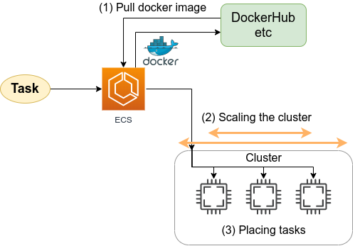
8. Hands-on #3: Deploying a question-answering bot on AWS
In the third hands-on session, we will implement a machine learning application using Docker and ECS. Specifically, we will create an automatic question-answering bot that generates answers to questions given by the client by performing natural language processing. By using ECS, we will build a system that dynamically controls the number of instances according to the number of jobs, and executes tasks in parallel.
|
In a typical machine learning workflow, the normal workflow is model training followed by inference (application to data). However, training models using EC2 clusters with GPUs is a little advanced, so it will be covered in the next sectopm (Section 9). This section introduces the parallelization of the inference using Fargate clusters, which can be implemented in a simpler program. This way you can familiarize yourself with the concepts of building clusters and managing tasks in the cloud. |
8.1. Fargate
Before getting into the hands-on exercuse, we need to learn about Fargate(Figure 43).

Let’s look again at Figure 42, which gives an overview of ECS. This figure shows a cluster under the control of ECS, and there are two choices which carry out the computation in the cluster: either EC2 or Fargate. In the case of using EC2, the instance is launched in the same way as described in the previous sections (Section 4, Section 6). However, the technical difficulty of creating and managing a compute cluster using EC2 is rather high, so we will explain it in the next section (Section 9).
Fargate is a mechanism for running container-based computational tasks, designed specifically for use in ECS.
In terms of running computation, its role is similar to that of EC2, but Fargate does not have a physical entity like an EC2 instance.
It means that, for example, logging in via SSH is basically not expected in Fargate, and there is no operations like "installing software".
In Fargate, all computation is executed via Docker containers.
Namely, to use Fargate, the user first prepares the Docker image, and then Fargate executes the computational task by using the docker run command.
When Fargate is specified as an ECS cluster, operations such as scaling can be built with a simple configuration and program.
Similar to EC2, Fargate allows you to specify the size of the CPU and memory as needed. At the time of writing, you can choose between 0.25 and 4 cores for vCPU power, and 0.5 and 30 GB for RAM (for details, see Official Documentation "Amazon ECS on AWS Fargate"]). Despite the ease of scaling clusters, Fargate does not allow for a large vCPU counts or RAM capacity, nor does it allow for the use of GPUs. as in EC2 instances.
So that was an overview of Fargate, but it may not be easy to understand it all in words. From here on, let us learn how to work with ECS and Fargate by writing a real program to deploy parallel computing system.
|
Strictly speaking, it is also possible to use a hybrid of EC2 and Fargate for the clusters attached to the ECS. |
8.2. Preparations
The source code of the hands-on is available on GitHub at handson/qa-bot.
To run this hands-on, it is assumed that the preparations described in the first hands-on (Section 4.1) have been completed. It is also assumed that Docker is already installed on your local machine.
|
For this hands-on, we will use a 1CPU/4GB RAM Fargate instance. Note that this will cost 0.025 $/hour to run the computation. |
8.3. A question-answering bot using Transformer
Let’s define more concretely the automatic question answering system that we will develop in this hands-on session. Assume that we are given the following context and question.
context: Albert Einstein (14 March 1879 – 18 April 1955) was a German-born theoretical physicist who developed the theory of relativity, one of the two pillars of modern physics (alongside quantum mechanics). His work is also known for its influence on the philosophy of science. He is best known to the general public for his mass–energy equivalence formula E = mc2, which has been dubbed \"the world's most famous equation\". He received the 1921 Nobel Prize in Physics \"for his services to theoretical physics, and especially for his discovery of the law of the photoelectric effect\", a pivotal step in the development of quantum theory.

question: In what year did Einstein win the Nobel prize?
The automatic answering system we are going to create will be able to find the correct answer to such a question, given the context. To make the problem a bit easier, the answer is selected from the string contained in the context. For example, for the above question, the system should return the following answer.
answer: 1921
While it is trivial for humans to understand such sentences, it is easy to imagine how difficult it would be for a computer to solve them. However, recent progress in natural language processing using deep learning has made remarkable progress, and it is possible to create models that can solve this problem with an extremely high accuracy.
In this hands-on, we will use the pre-trained language model provided by huggingface/transformers. This model is supported by a natural language processing model called Transformer We packaged this model in a Docker image, and the image is available at the author’s Docker Hub repository. Before we start designing the cloud system, let’s test this Docker image on the local machine.
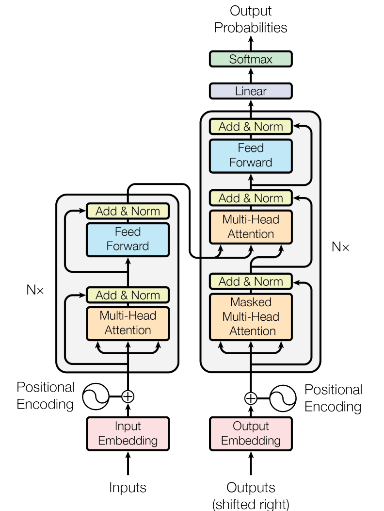
|
Since we are using a pre-trained model, all we need to do is to feed the given input into the model and make a prediction (inference). Since the inference operations can be done quickly enough on a CPU alone, we will not use a GPU in this hands-on session to reduce the cost and simplify the implementation. In general, training is much more computationally expensive for neural nets, and the GPU is more powerful in such cases. |
Use the following command to download (pull) the Docker image to your local machine.
$ docker pull tomomano/qabot:latestNow, let’s submit a question to this Docker image. First, define the context and question as command line variables.
$ context="Albert Einstein (14 March 1879 – 18 April 1955) was a German-born theoretical physicist who developed the theory of relativity, one of the two pillars of modern physics (alongside quantum mechanics). His work is also known for its influence on the philosophy of science. He is best known to the general public for his mass–energy equivalence formula E = mc2, which has been dubbed the world's most famous equation. He received the 1921 Nobel Prize in Physics for his services to theoretical physics, and especially for his discovery of the law of the photoelectric effect, a pivotal step in the development of quantum theory."
$ question="In what year did Einstein win the Nobel prize ?"
Then, use the following command to run the container.
$ docker run tomomano/qabot "${context}" "${question}" foo --no_saveThe Docker image we prepared accepts the context as the first argument and the question as the second argument. The third and fourth arguments are for implementation purposes when deploying to the cloud, so don’t worry about them for now.
When you execute this command, you should get the following output.
{'score': 0.9881729286683587, 'start': 437, 'end': 441, 'answer': '1921'}
"score" is a number that indicates the confidence level of the answer, in the range [0,1]. "start" and "end" indicate the starting and ending position in the context where the answer is, and "answer" is the string predicted as the answer. Notice that the correct answer, "1921", was returned.
Let us ask a more difficult question.
$ question="Why did Einstein win the Nobel prize ?"
$ docker run tomomano/qabot "${context}" "${question}" foo --no_save
Output:
{'score': 0.5235594527494207, 'start': 470, 'end': 506, 'answer': 'his services to theoretical physics,'}
This time, the score is 0.52, indicating that the bot is a little unsure of the answer, but it still got the right answer.
As you can see, by using a language model supported by deep learning, we have been able to create a Q&A bot that can be useful in practical applications. In the following sections, we will design a system that can automatically respond to a large number of questions by deploying this program in the cloud.
|
The question & answering system used in this project uses a Transformer-based language model called DistilBERT. Interested readers can refer to original paper. For documentation of the DistilBert implementation by huggingface/transformers, see official documentation. |
|
The source code for the Q-A bot Docker image is available at GitHub. |
8.4. Reading the application source code
Figure 45 shows an overview of the application we are creating in this hands-on.
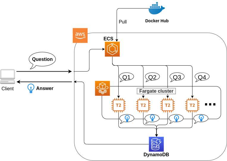
The summary of the system design is as follows:
-
The client sends a question to the application on AWS.
-
The task to solve the submitted question is handled by ECS.
-
ECS downloads an image from Docker Hub.
-
ECS then launches a new Fargate instance in the cluster and places the downloaded Docker image in this new instance
-
One Fargate instance is launched for each question so that multiple questions can be processed in parallel.
-
-
The job is executed. The results of the job (the answers to the questions) are written to the DynamoDB database.
-
Finally, the client reads the answers to the questions from DynamoDB.
Now let us take a look at the main application code (handson/qa-bot/app.py).
 1
 2
 3
 4
 5
 6
 7
 8
 9
10
11
12
13
14
15
16
17
18
19
20
21
22
23
24
25
26
27
28
29
30
31
32
33
34
35
36
37
38
39
40
41
42
43
44
45
46
47
48
49
50
51
52
class EcsClusterQaBot(Stack):

    def __init__(self, scope: Construct, construct_id: str, **kwargs) -> None:
        super().__init__(scope, construct_id, **kwargs)

        (1)
        # dynamoDB table to store questions and answers
        table = dynamodb.Table(
            self, "EcsClusterQaBot-Table",
            partition_key=dynamodb.Attribute(
                name="item_id", type=dynamodb.AttributeType.STRING
            ),
            billing_mode=dynamodb.BillingMode.PAY_PER_REQUEST,
            removal_policy=cdk.RemovalPolicy.DESTROY
        )

        (2)
        vpc = ec2.Vpc(
            self, "EcsClusterQaBot-Vpc",
            max_azs=1,
        )

        (3)
        cluster = ecs.Cluster(
            self, "EcsClusterQaBot-Cluster",
            vpc=vpc,
        )

        (4)
        taskdef = ecs.FargateTaskDefinition(
            self, "EcsClusterQaBot-TaskDef",
            cpu=1024, # 1 CPU
            memory_limit_mib=4096, # 4GB RAM
        )

        # grant permissions
        table.grant_read_write_data(taskdef.task_role)
        taskdef.add_to_task_role_policy(
            iam.PolicyStatement(
                effect=iam.Effect.ALLOW,
                resources=["*"],
                actions=["ssm:GetParameter"]
            )
        )

        (5)
        container = taskdef.add_container(
            "EcsClusterQaBot-Container",
            image=ecs.ContainerImage.from_registry(
                "tomomano/qabot:latest"
            ),
        )
| 1 | Here, we are preparing a database to write the results of the answers. DynamoDB will be covered in the sections on the serverless architecture (Section 11 and Section 12), so don’t worry about it for now. |
| 2 | Here, we define a VPC, as we did in Hands-on #1 and #2. |
| 3 | Here, we define ECS clusters. A cluster is a pool of virtual servers, and multiple virtual instances are placed in a cluster. |
| 4 | Here, we define the tasks to be executed (task definition). |
| 5 | Here, we define the Docker image to be used for executing the task. |
8.4.1. ECS and Fargate
Let’s take a closer look at the code for ECS and Fargate.
 1
 2
 3
 4
 5
 6
 7
 8
 9
10
11
12
13
14
15
16
17
cluster = ecs.Cluster(
    self, "EcsClusterQaBot-Cluster",
    vpc=vpc,
)

taskdef = ecs.FargateTaskDefinition(
    self, "EcsClusterQaBot-TaskDef",
    cpu=1024, # 1 CPU
    memory_limit_mib=4096, # 4GB RAM
)

container = taskdef.add_container(
    "EcsClusterQaBot-Container",
    image=ecs.ContainerImage.from_registry(
        "tomomano/qabot:latest"
    ),
)
In the line starting with cluster =, a empty ECS cluster is created.
Then, taskdef=ecs.FargateTaskDefinition creates a new task definition.
Task definition specifies all necessary information to run the task, including the CPU and RAM size.
Here, we will use 1 CPU and 4GB RAM to execute the task.
Also, note that the task defined this way uses one instance per task.
Lastly, in the line starting with container =, we are supplying the link to the Docker image to the task definition.
Here, we specify to download an image called tomomano/qabot from Docker Hub.
With this just a few lines of code, we can create an ECS cluster which automatically executes the task scheduling and cluster scaling.
|
In the above code, notice the line which says
|
8.5. Deploying the application
Now that we understand the application source code, let’s deploy it.
The deployment procedure is almost the same as the previous hands-on.
Here, only the commands are listed (lines starting with # are comments).
If you have forgotten the meaning of each command, review the first hands-on.
You should not forget to set the access key (Section 14.3).
# move to the project directory
$ cd handson/qa-bot

# create venv and install dependent libraries
$ python3 -m venv .env
$ source .env/bin/activate
$ pip install -r requirements.txt

# Deploy!
$ cdk deploy
If the deployment is successful, you should see an output like Figure 46.
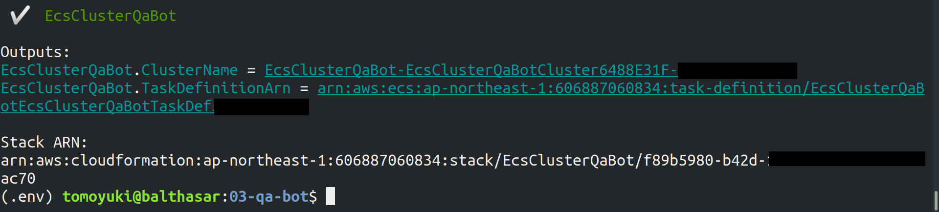
cdk deployLet’s log in to the AWS console and check the contents of the deployed stack.
From the console, go to the ECS page, and you should see a screen like Figure 47.
Find the cluster named EcsClusterQaBot-XXXX.
Cluster is a unit that binds multiple virtual instances together, as explained earlier.
In the Figure 47, check that under the word FARGATE it says 0 Running tasks and 0 Pending tasks.
At this point, no tasks were submitted, so the numbers are all zero.
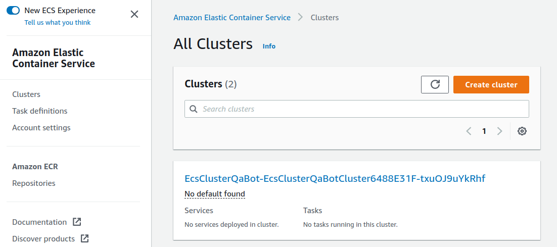
Next, find the item Task Definitions in the menu bar on the left of this screen, and click on it.
On the destination page, find the item EcsClusterQaBotEcsClusterQaBotTaskDefXXXX and open it.
Scroll down the page, and you will find the information shown in Figure 48.
You can check the amount of CPU and memory used, as well as the settings related to the execution of the Docker container.
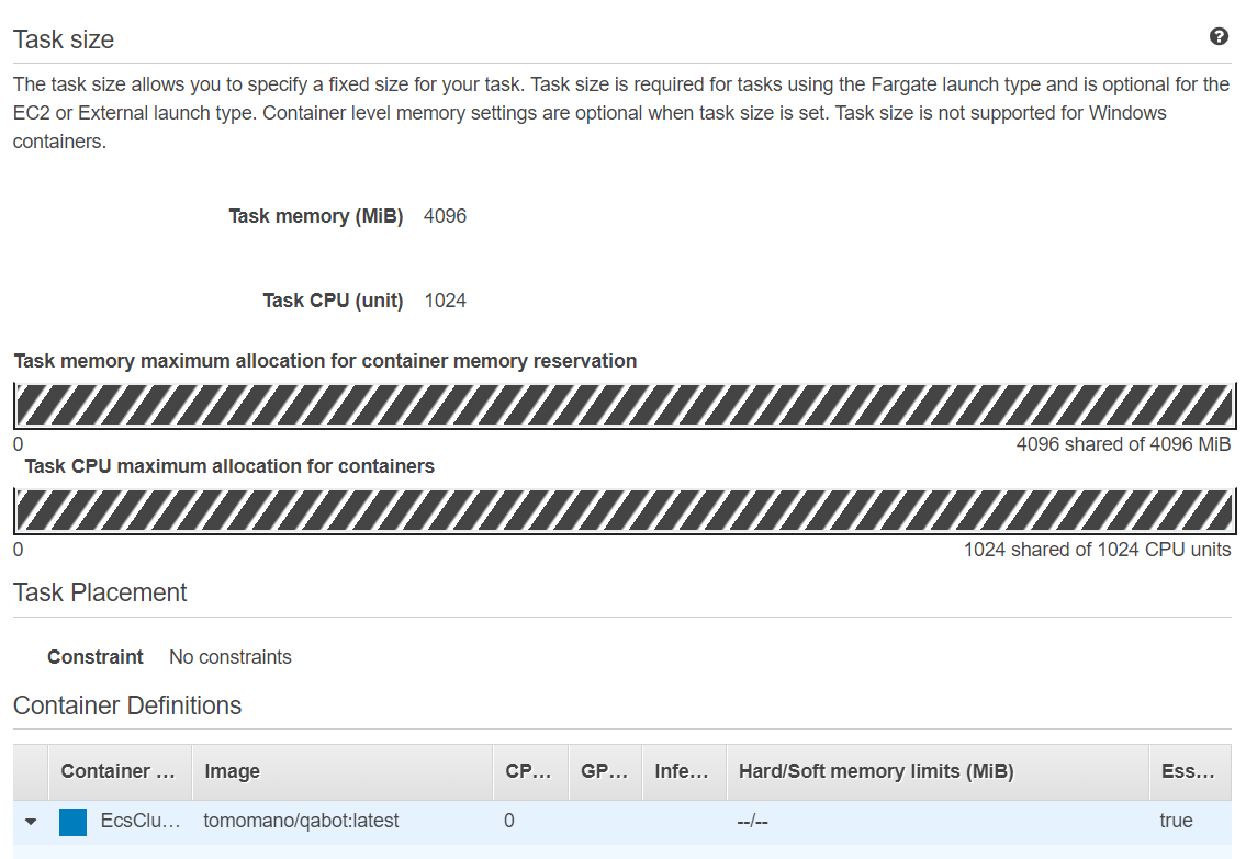
8.6. Executing a task
Now, let’s submit a question to the cloud!
Submitting a task to ECS is rather complicated, so I prepared a program (run_task.py) to simplify the task submission.
(handson/qa-bot/run_task.py).
With the following command, you can submit a new question to the ECS cluster.
$ python run_task.py ask "A giant peach was flowing in the river. She picked it up and brought it home. Later, a healthy baby was born from the peach. She named the baby Momotaro." "What is the name of the baby?"|
In order to run |
Following "ask" parameter, we supply context and questsions, in this order, as the arguments.
When you run this command, you will see the output "Waiting for the task to finish…", and you will have to wait for a while to get an answer. During this time, ECS accepts the task, launches a new Fargate instance, and places the Docker image on the instance. Let’s monitor this sequence of events from the AWS console.
Go back to the ECS console screen, and click on the name of the cluster (EcsClusterQaBot-XXXX).
Next, open the tab named "Tasks" (Figure 49).
You will see a list of running tasks.
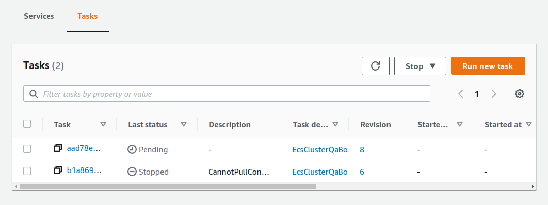
As you can see in Figure 49, the "Last status = Pending" indicates that the task is being prepared for execution at this point. It takes about 1-2 minutes to launch the Fargate instance and deploy the Docker image.
After waiting for a while, the status will change to "RUNNING" and the computation will start. When the computation is finished, the status changes to "STOPPED" and the Fargate instance is automatically shut down by ECS.
From the Figure 49 screen, click on the task ID in the "Task" column to open the task detail screen (Figure 50). The task information such as "Last status" and "Platform version" is displayed. You can also view the execution log of the container by opening the "Logs" tab.
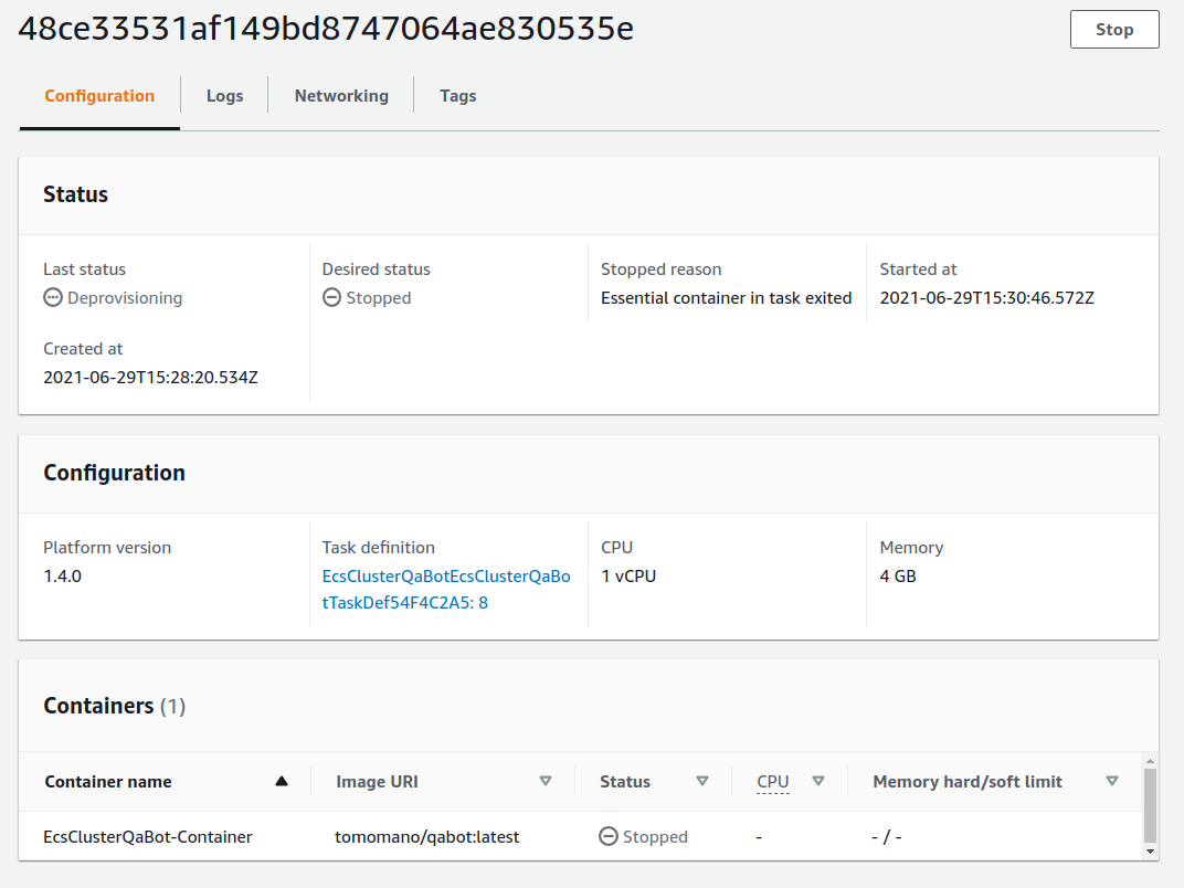
Now, coming back to the command line where you ran run_task.py, you should see an output like Figure 51.
The correct answer, "Momotaro", has been returned!
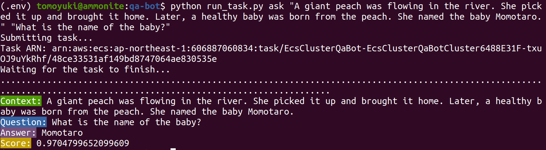
8.7. Executing tasks in parallel
The application we have designed here can handle many questions at the same time by using ECS and Fargate.
Now, let’s submit many questions at once, and observe the behavior of ECS cluster.
By adding the option ask_many to run_task.py, you can send multiple questions at once.
The questions are defined in
handson/qa-bot/problems.json.
Run the following command.
$ python run_task.py ask_manyAfter executing this command, go to the ECS console and look at the list of tasks (Figure 52). You can see that multiple Fargate instances have been launched and tasks are being executed in parallel.
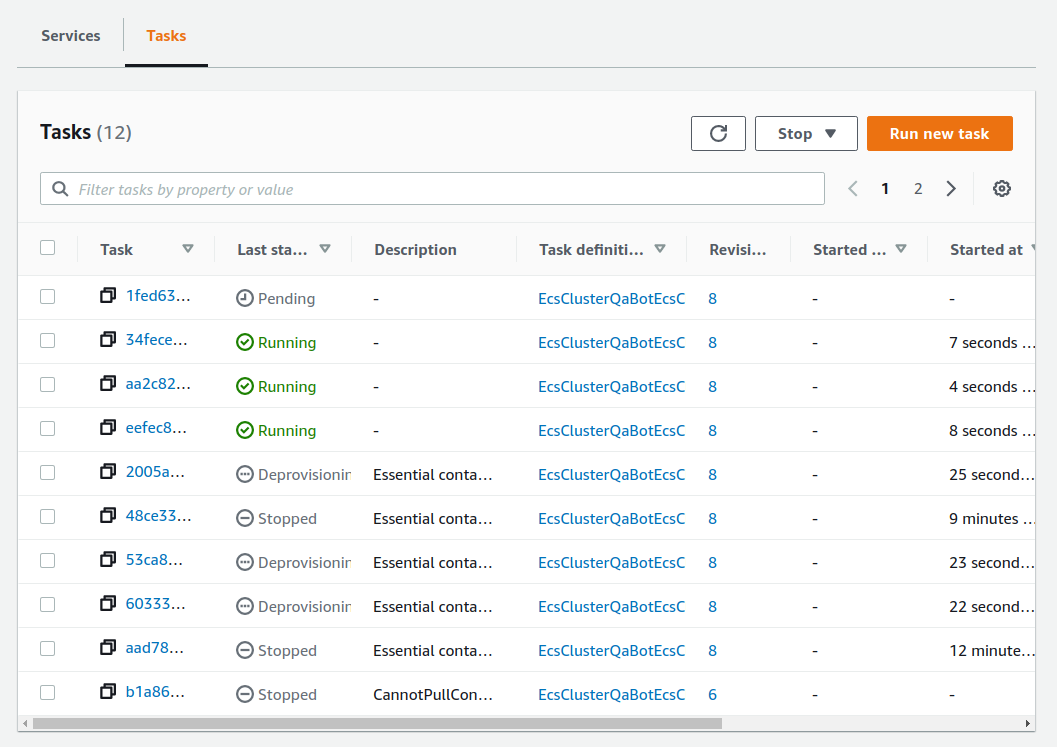
Make sure that the status of all tasks is "STOPPED", and then get the answer to the question. To do so, execute the following command.
$ python run_task.py list_answersAs a result, you will get an output like Figure 53. You can see that the bot was able to answer complex text questions with a suprisingly high accuracy.
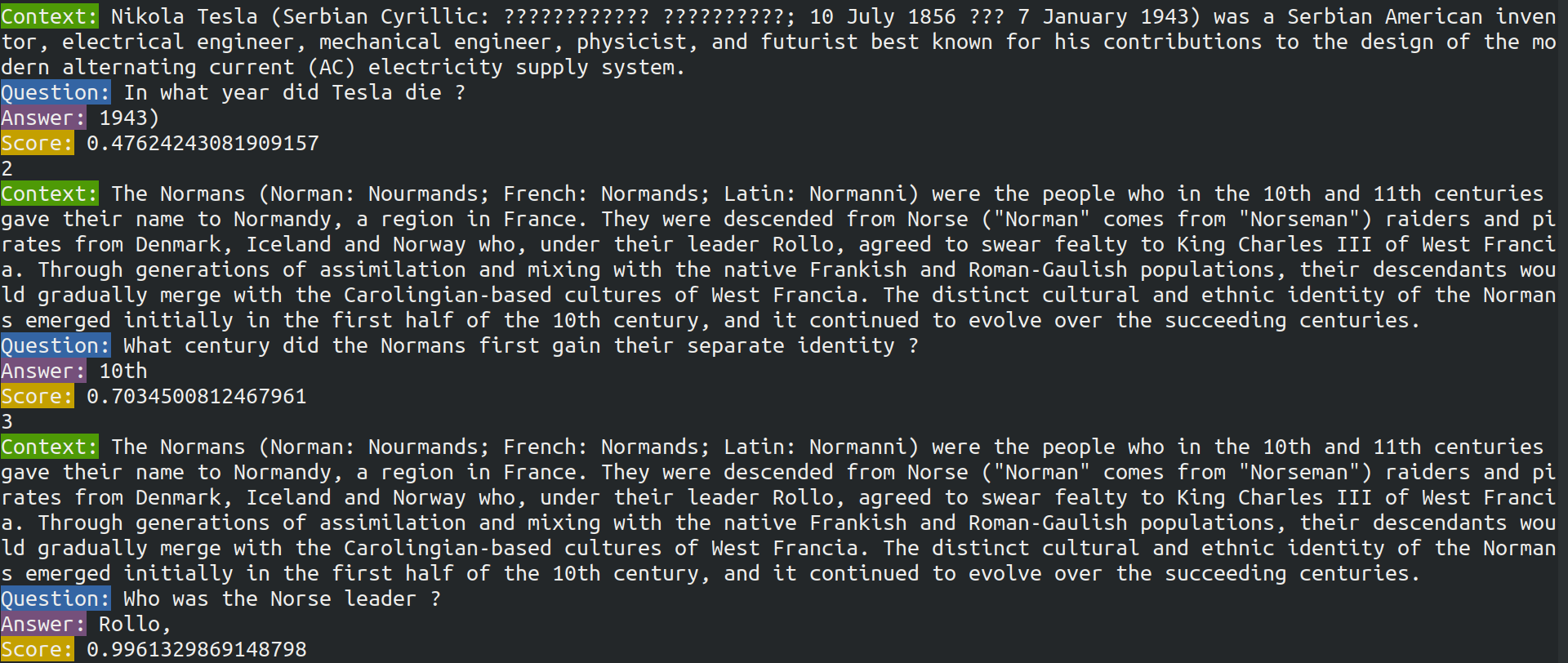
$ python run_task.py list_answers|
If you keep submitting questions with |
Congratulations! You have managed to create a system that can automatically generate answers to questions using deep learning language models! Importantly, it is a highly scalable system that can handle hundreds of questions simultaneously. We didn’t prepare a GUI (Graphical User Interface) this time, but if we add a simple GUI to this system, it could be operated as a very nice web service. We didn’t add GUI to this cloud system, but with such a tweaking, this system is already useful enough for various purposes.
8.8. Deleting the stack
This concludes the third hands-on session. Finally, we must delete the stack.
To delete the stack, login to the AWS console and click the DELETE button on the CloudFormation screen. Alternatively, you can execute the following command from the command line.
$ cdk destroy9. Hands-on #4: Using AWS Batch to Parallelize Hyperparameter Search for Machine Learning
In the third hands-on session, we built an automatic question answering system using ECS and Fargate. Despite its simplicity, we were able to build a system where jobs are executed in parallel when multiple questions are sent. There, we built the application using a pre-tained language model. Generally speaking, though, the first step in a machine learning workflow should be to train your own models. Therefore, in the fourth hands-on session, we will consider parallelizing and accelerating the training of machine learning models using the cloud.
In particular, we will focus on hyperparameter optimization in deep learning. Hyperparameters are parameters outside the weights of the neural network that are optimized by gradient descent, including those related to the architecture of the network such as the width and depth of the layers, and those related to the parameter optimization method such as the learning rate and momentum. Tuning the hyperparameters is a very important task in deep learning. However, it requires a lot of computation time because the neural network needs to be trained many times while changing the conditions little by little. In research and development, exploring a large number of possible models is an important factor in determining productivity, and the problem of solving hyperparameter search quickly is of great interest. In this hands-on, we will learn how to solve this problem by training neural networks in parallel using the powerful computing resources of the cloud.
9.1. Auto scaling groups (ASG)
Before we get into the hands-on, you need to be familiar with the technique of EC2, called Auto scaling groups (ASG).
Please take a look back at Figure 42, which gives an overview of ECS. As explained in the previous chapter (Section 8), EC2 and Fargate can be selected as the computational resource in ECS clusters. Fargate was described in the previous chapter. Using Fargate, we were able to build a highly scalable computing environment with a simple setup. However, there were some limitations, such as not being able to use GPUs. By defining a computing environment that is based on EC2, although the programming complexity increases, we can build clusters with GPUs and other more advanced and complex configurations.
A service called ASG is deployed in an EC2 cluster. An ASG constitutes a cluster by grouping multiple EC2 instances into logical units. ASGs are responsible for scaling, such as launching new instances in the cluster or stopping instances that are no longer needed. An important concept in ASG is the parameters callled desired capacity, minimum capacity, and maximum capacity. The minimum capacity and maximum capacity are parameters that specify the minimum and maximum number of instances that can be placed in a cluster, respectively. The former keeps the instances idle even when the cluster is not under load, so it can act as a buffer when the load suddenly increases. The latter prevents an excessive number of instances from being launched when the load increases unexpectedly, and serves to set an upper limit on the economic cost.
The desired capacity specifies the number of instances required by the system at a given time. The desired capacity can be set based on a fixed schedule, such as increasing or decreasing the number of instances according to a 24-hour rhythm (e.g., more during the day and less at night). Alternatively, the desired capacity can be dynamically controlled according to the load on the entire cluster. The rules that define the criteria for scaling the cluster are called scaling policies. For example, we can assume a scaling policy which maintains the utilization (load) of the entire cluster at 80% at all times. In this case, the ASG automatically removes instances from the cluster when the load of the entire cluster falls below 80%, and adds instances when the load exceeds 80%s.
After considering the above parameters, the user creates an ASG. Once ASG is created, one needs to write a program to link ASG with the ECS, which defines EC2-based ECS cluster.
9.2. AWS Batch

As explained earlier, it is possible to construct a desired computation cluster by combining ECS and ASG. However, ECS and ASG require complicated settings, which makes programming quite tedious for both beginners and experienced users. To solve this problem, there is a service that automates the design of clusters using ECS and ASG. That service is AWS Batch.
AWS Batch, as the name implies, is designed for batch jobs (i.e., independent operations with different input data that are executed repeatedly). Many scientific calculations and machine learning can be considered as batch calculations. For example, you can run multiple simulations with different initial parameters. The advantage of using AWS Batch is that the scaling of the cluster and the allocation of jobs are all done automatically, giving the users a system where they can submit a large number of jobs without worrying about the implementation details of the cloud. However, it is important to know that the ECS/ASG/EC2 triad is working in concert behind the scenes.
In AWS Batch, the following concept is defined to facilitate job submission and management (Figure 55). First, a job is a unit of computation executed by AWS Batch. Job definitions define the specification of a job, including the address of the Docker image to be executed, the amount of CPU and RAM to be allocated, and environment variables. Each job is executed based on the job definition. When a job is executed, it is placed in job queues. Job queue is a queue of jobs waiting to be executed, and the first job in the queue is executed first. In addition, multiple queues can be arranged, and each queue can be assigned a priority value, so that jobs in the queue with the highest priority are executed first. Compute environment is a concept that is almost synonymous with the cluster, and refers to the location where computations are executed (i.e. group of EC2 or Fargate instances). In the compute environment, one needs to specify the EC2 instance types to use, and a simple scaling policy, such as the upper and lower limit on the number of instances. Job queues monitor the availability of the compute environment and place jobs to the compute environment according to the availability.
These are the concepts that you need to understand when using AWS Batch. To make a better sense of these concepts, let us actually construct an application using AWS Batch.
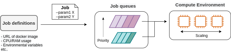
|
EC2 or Fargate? When configuring a cluster in ECS, we explained that there are two options for performing calculations: EC2 and Fargate. Each has its own advantages and disadvantages, but which one should be used in which case? To examine this, let’s first look at Table 5. This is a summary of the characteristics of EC2 and Fargate. Please note that it is heavily coarse-grained for the sake of explanation.
As we have seen so far, EC2 has high computing power in a single instance, with a large maximum number of CPUs and memory size, and the ability to use GPUs. In contrast, the maximum number of CPUs for a single instance of Fargate is capped at four cores. On the other hand, the time required to launch an instance is much faster in Fargate, which allows for more agile scaling of the cluster. Fargate also has higher flexibility when submitting tasks to the cluster. Flexibility refers to the situation where, for example, two or more containers can be run on a single instance. Such a design is often used to maximize the number of tasks per unit CPU. In terms of programming complexity, Fargate is generally simpler to implement. As described above, EC2 and Fargate have complementary characteristics, and the optimal computing environment must be considered carefully depending on the use cases. It is also possible to define a hybrid cluster that uses both EC2 and Fargate, and such an option is often used. |
9.3. Preparations
The hands-on source code is available on GitHub at handson/aws-batch.
To run this hands-on, it is assumed that the preparations described in the first hands-on (Section 4.1) have been completed. It is also assumed that Docker is already installed on your local machine.
|
Since this hands-on uses |
|
As noted in Section 6.1, before starting this hands-on, check the launch limit of G-type instances from the EC2 dashboard of the AWS console. If the limit is 0, you need to apply for increase of the limit. Also refer to Section 9.5 for related information. |
9.4. Revisiting MNIST handwritten digit recognition task
At the beginning of this hands-on, we mentioned that we would be covering hyperparameter tuning in machine learning. As the simplest example, let’s take the MNIST digit recognition problem again, which was covered in Section 6.7. In Section 6.7, we trained the model using arbitrarily chosen hyperparameters. The hyperparameters used in the program include learning rate and momentum in stochastic gradient descent (SGD) algorithm. In the code, the following lines correspond to them.
optimizer = optim.SGD(model.parameters(), lr=0.01, momentum=0.5)The learning rate (lr=0.01) and momentum (momentum=0.5) used here are arbitrarily chosen values, and we do not know if these are the best values.
This choice may happen to be the best, or there may be other hyperparameter pairs that give higher accuracy.
To answer this question, let’s perform a hyperparameter search.
In this article, we will take the simplest approach: hyperparameter search by grid search.
First, let’s run the Docker image used in this hands-on session locally.
The source code of the Docker image can be found on GitHub at handson/aws-batch/docker. It is based on the program we introduced in Section 6.7, with some minor changes made for this handson. Interested readers are encouraged to read the source code as well.
As an exercise, let’s start by building this Docker image on your local machine.
Go to the directory where the Dockerfile is stored, and build the image with the tag mymnist.
$ cd handson/aws-batch/docker
$ docker build -t mymnist .|
If you get an error with |
|
Instead of building the image yourself, you can pull it from Docker Hub. In this case, execute the following command. |
When the image is ready, start the container with the following command and run MNIST training.
$ docker run mymnist --lr 0.1 --momentum 0.5 --epochs 10This command will start optimizing the neural network using the specified hyperparameters (learning rate given by --lr and momentum given by --momentum).
The maximum number of epochs to train is specified by --epochs parameter.
You will see decrease of loss values on the command line, just as we saw in Section 6 (Figure 56).
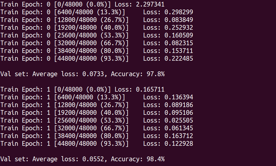
If you use the above command, the computation will be performed using the CPU. If your local computer is equipped with a GPU and you have configured nvidia-docker, you can use the following command to run the computation using the GPU.
$ docker run --gpus all mymnist --lr 0.1 --momentum 0.5 --epochs 10In this command, the parameter --gpus all has been added.
You can see that the loss of the training data monotonically decreases as the number of epochs increases, regardless of whether it is run on CPU or GPU. On the other hand, you will notice that loss and accuracy of the validation data do not improve further after decreasing to a certain level. The actual plot of this behaviour should look like Figure 57.
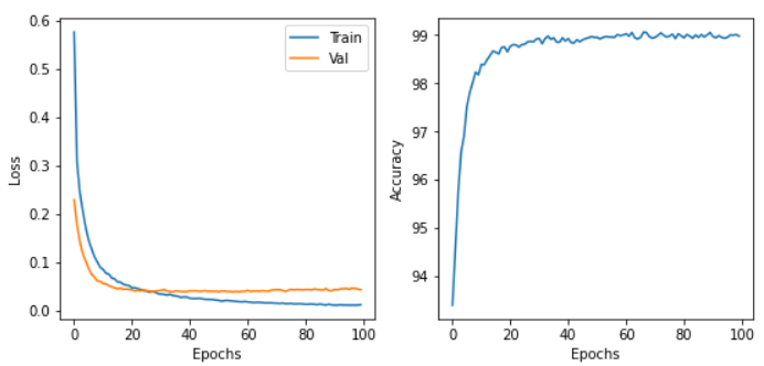
This is a phenomenon called overfitting, which indicates that the neural network is over-fitted to the training data and the accuracy (generalization performance) for data outside the training data is not improved. To deal with such cases, a technique called early stopping is known. In early stopping, we track the loss of the validation data, and stop learning at the epoch when it turns from decreasing to increasing. Then we adopt the weight parameters at that epoch. In this hands-on session, we will use early stopping technique to determine the end of training and evaluate the performance of the model.
|
In the MNIST handwriting dataset, 60,000 images are given as training data and 10,000 images as test data. In the code used in this hands-on session, 48,000 images (80% of the training data) are used as training data, and the remaining 12,000 images are used as validation data. For details, please refer to the source code. |
9.5. Reading the application source code
Figure 58 shows an overview of the application we are creating in this hands-on.
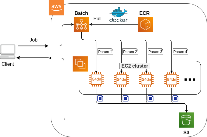
The summary of the system design is as follows:
-
The client submits a job to AWS Batch with a given set of hyperparameters.
-
When Batch receives the job, it performs the computation on a cluster consisting of EC2
-
A
g4dn.xlargeinstance is launched in the cluster. -
Docker images are retrieved from the Elastic Container Registry (ECR) in AWS.
-
When multiple jobs are submitted, enough number of instances are launched and jobs are executed in parallel.
-
The results of the computation by each job are stored in S3.
-
Finally, the client downloads the results from S3 and decides the best set of hyperparameters.
Let us take a look at the application source code (handson/aws-batch/app.py).
 1
 2
 3
 4
 5
 6
 7
 8
 9
10
11
12
13
14
15
16
17
18
19
20
21
22
23
24
25
26
27
28
29
30
31
32
33
34
35
36
37
38
39
40
41
42
43
44
45
46
47
48
49
50
51
52
53
54
55
56
57
58
59
60
61
62
63
64
65
66
67
68
69
70
71
72
73
74
75
76
77
78
79
class SimpleBatch(Stack):

    def __init__(self, scope: Construct, construct_id: str, **kwargs) -> None:
        super().__init__(scope, construct_id, **kwargs)

        (1)
        bucket = s3.Bucket(
            self, "bucket",
            removal_policy=cdk.RemovalPolicy.DESTROY,
            auto_delete_objects=True,
        )

        vpc = ec2.Vpc(
            self, "vpc",
            # other parameters...
        )

        (2)
        managed_env = batch_alpha.ComputeEnvironment(
            self, "managed-env",
            compute_resources=batch_alpha.ComputeResources(
                vpc=vpc,
                allocation_strategy=batch_alpha.AllocationStrategy.BEST_FIT,
                desiredv_cpus=0,
                maxv_cpus=64,
                minv_cpus=0,
                instance_types=[
                    ec2.InstanceType("g4dn.xlarge")
                ],
            ),
            managed=True,
            compute_environment_name=self.stack_name + "compute-env"
        )

        (3)
        job_queue = batch_alpha.JobQueue(
            self, "job-queue",
            compute_environments=[
                batch_alpha.JobQueueComputeEnvironment(
                    compute_environment=managed_env,
                    order=100
                )
            ],
            job_queue_name=self.stack_name + "job-queue"
        )

        (4)
        job_role = iam.Role(
            self, "job-role",
            assumed_by=iam.CompositePrincipal(
                iam.ServicePrincipal("ecs-tasks.amazonaws.com")
            )
        )
        # allow read and write access to S3 bucket
        bucket.grant_read_write(job_role)

        (5)
        repo = ecr.Repository(
            self, "repository",
            removal_policy=cdk.RemovalPolicy.DESTROY,
        )

        (6)
        job_def = batch_alpha.JobDefinition(
            self, "job-definition",
            container=batch_alpha.JobDefinitionContainer(
                image=ecs.ContainerImage.from_ecr_repository(repo),
                command=["python3", "main.py"],
                vcpus=4,
                gpu_count=1,
                memory_limit_mib=12000,
                job_role=job_role,
                environment={
                    "BUCKET_NAME": bucket.bucket_name
                }
            ),
            job_definition_name=self.stack_name + "job-definition",
            timeout=cdk.Duration.hours(2),
        )
| 1 | Here, we prepare an S3 bucket to store the results of the jobs. |
| 2 | Here, we define the compute environment.
The g4dn.xlarge instance is used, and the maximum number of vCPU usage is specified as 64.
The minimum vCPU is 0. |
| 3 | This part defines the job queue associated with the compute environment created in <2>. |
| 4 | Here we define the IAM role so that the job can write results to S3 (IAM is a mechanism to manage the permissions of resources. See Section 13.2.5 for details). |
| 5 | This line defines the ECR for deploying the Docker image. |
| 6 | Here we create the job definition.
In the code, we specify each job to consume 4 vCPU and 12000 MB (=12GB).
It also sets the environment variables (BUCKET_NAME) that will be used by the Docker container.
In addition, the IAM created in <4> has been attatched. |
|
Each There is one point to note here.
AWS sets an upper limit for the number of instances that can be launched in EC2 for each account.
You can check this limit by logging into the AWS console and clicking 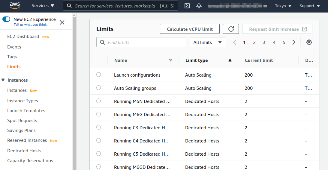
Figure 59. Checking the limits from EC2 console
|
9.6. Deploying the stack
Now that we understand the application source code, let’s deploy it.
The deployment procedure is almost the same as the previous hands-on.
Here, only the commands are listed (lines starting with # are comments).
If you have forgotten the meaning of each command, review the first hands-on.
You should not forget to set the access key (Section 14.3).
# move to the project directory
$ cd handson/aws-batch

# create venv and install dependent libraries
$ python3 -m venv .env
$ source .env/bin/activate
$ pip install -r requirements.txt

# Deploy!
$ cdk deploy
After confirming that the deployment has been done successfully, let’s log in to the AWS console and check the deployed stack.
Type batch in the search bar to open the AWS Batch management console (Figure 60).
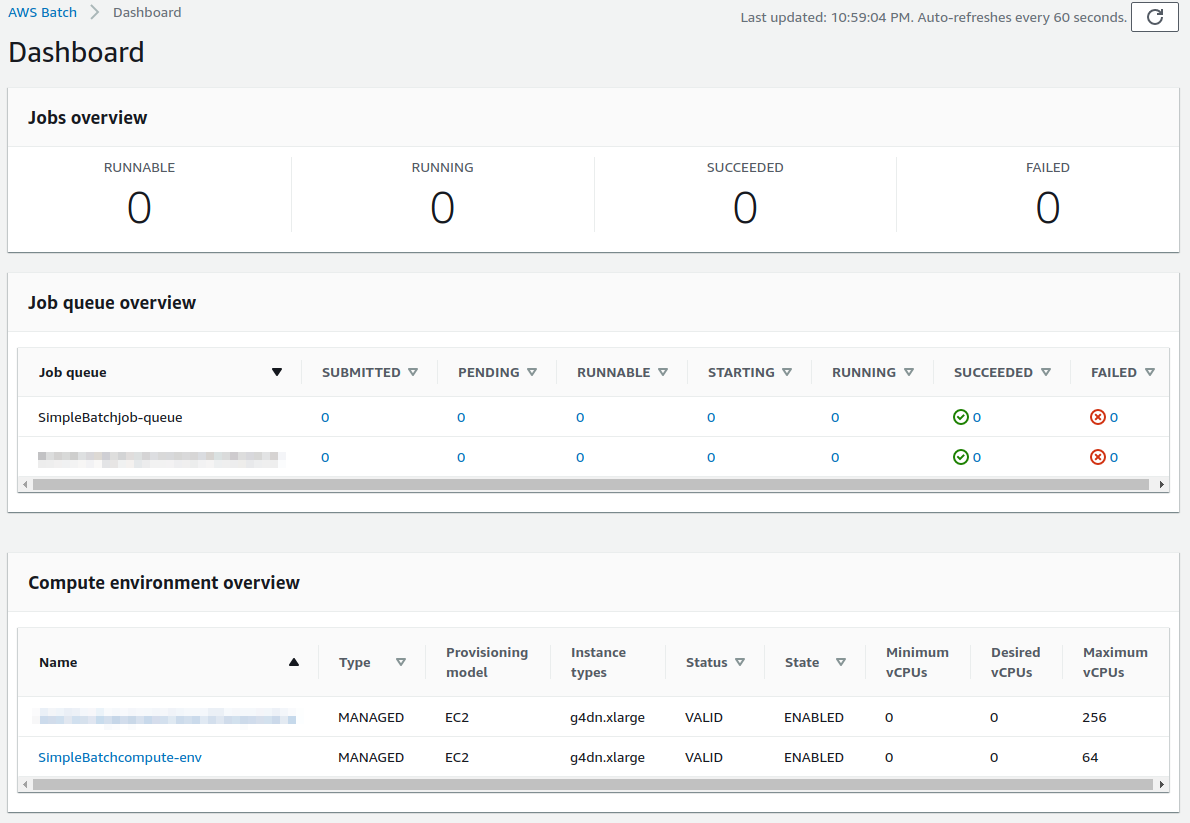
The first thing you should look at is the item named SimpleBatchcompute-env in the "compute environment overview" at the bottom of the screen.
Compute environment is the environment (or cluster) in which computations will be executed, as described earlier.
As specified in the program, g4dn.xlarge is shown as the instance type to be used.
You can also see that Minimum vCPUs is set to 0 and Maximum vCPUs is set to 64.
In addition, Desired vCPUs is set to 0 because no job is running at this time.
If you want to see more detailed information about the compute environment, click on the name to open the detail screen.
Next, pay attention to the item SimpleBatch-queue in the "job queue overview".
Here, you can see a list of jobs waiting for execution, jobs in progress, and jobs that have completed execution.
You can see that there are columns such as PENDING, RUNNING, SUCCEEDED, FAILED and so on.
As the job progresses, the state of the job transitions according to these columns.
We’ll come back to this later when we actually submit the job.
Finally, let’s check the job definition.
Select Job definitions from the menu on the left side of the screen, and find and open the SimpleBatchjob-definition on the next screen.
From here, you can see the details of the job definition (Figure 61).
Among the most important information, vCPUs, Memory, and CPU define the amount of vCPU, memory, and GPU allocated to Docker, respectively.
In addition, Image specifies the Docker image to be used for the job.
Here, it refers to the ECR repository.
Currently, this ECR is empty.
The next step is to deploy the image to this ECR.
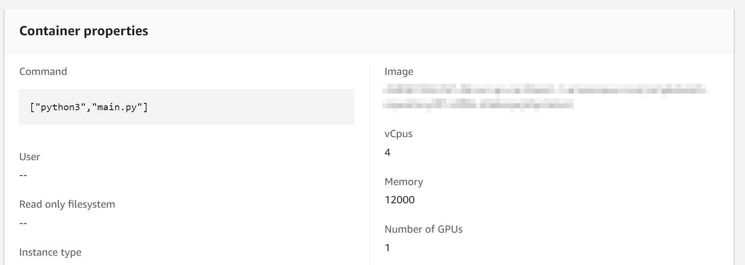
9.7. Deploying Docker image on ECR
In order for Batch to execute a job, it needs to download (pull) a Docker image from a specified location. In the previous hands-on (Section 8), we pulled the image from Docker Hub, which is set to public. In this hands-on, we will adopt the design of deploying images in ECR (Elastic Container Registry), a image registry provided by AWS. The advantage of using ECR is that you can prepare a private space for images that only you can access. Batch executes its tasks by pulling images from the ECR (Figure 58).
In the source code, the following part defines the ECR.
(1)
repo = ecr.Repository(
    self, "repository",
    removal_policy=cdk.RemovalPolicy.DESTROY,
)

job_def = batch_alpha.JobDefinition(
    self, "job-definition",
    container=batch_alpha.JobDefinitionContainer(
        image=ecs.ContainerImage.from_ecr_repository(repo), (2)
        ...
    ),
    ...
)| 1 | This creates a new ECR. |
| 2 | In the job definition, we specify that the image should be retrieved from the ECR created in <1>. At the same time, the job definition is automatically granted access rights to the ECR through IAM. |
After the first deployment, the ECR is empty. You need to push the Docker image that you use for your application to ECR.
To do so, first open the ECR screen from the AWS console (type Elastic Container Registry in the search bar).
Select the Private tab and you will find a repository named simplebatch-repositoryXXXX (Figure 62).
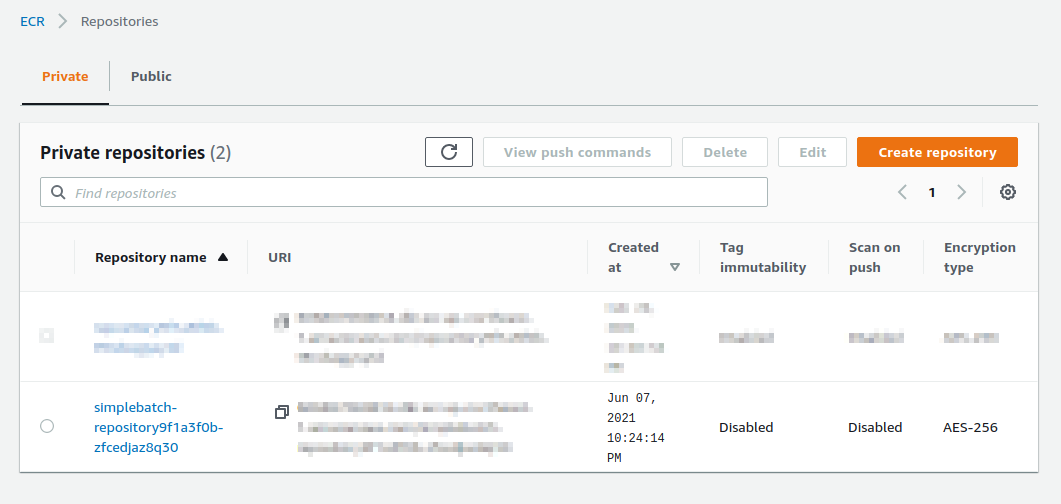
Next, click on the name of the repository to go to the repository details page.
Then, click the View push commands button on the upper right corner of the screen.
This will bring up a pop-up window like Figure 63.
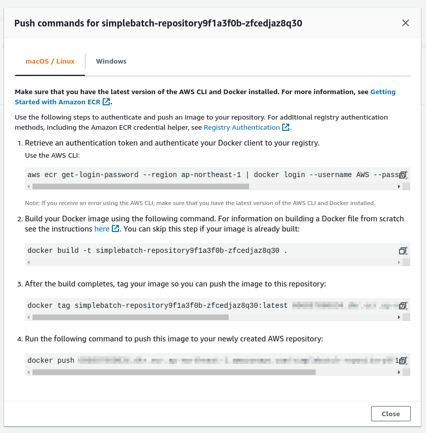
You can push your Docker image to ECR by executing the four commands shown in this pop-up window in order.
Before pushing, make sure your AWS credentials are set.
Then, navigate to the directory named docker/ in the hands-on source code.
Then, execute the commands displayed in the pop-up window in order from the top.
|
If you look at the second command that pops up, you will see |
The fourth command may take a few minutes as it uploads several gigabytes of images to ECR, but when it completes, the image has been successfully placed in ECR. If you look at the ECR console again, you can see that the image has indeed been placed (Figure 64). This completes the final preparations for executing a job using AWS Batch.
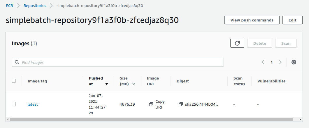
9.8. Submitting a single job
Now, we demonstrate how to submit a job to AWS Batch.
In the notebook/ directory of the hands-on source code, there is a file named
run_single.ipynb
(.ipynb is the file extension of Jupyter notebook).
We will open this file from Jupyter notebook.
In this hands-on, Jupyter Notebook server is already installed in the virtual environment by venv.
We can launch Jupyter Notebook server from the local machine by the following command.
# Make sure that you are in a virtual environment
(.env) $ cd notebook
(.env) $ jupyter notebook
After Jupyter Notebook server is started, open run_single.ipynb.
The first cell [1], [2], [3] defines a function to submit a job to AWS Batch (submit_job()).
 1
 2
 3
 4
 5
 6
 7
 8
 9
10
11
12
13
14
15
16
17
18
19
20
21
22
23
24
25
26
27
28
29
# [1]
import boto3
import argparse

# [2]
# AWS 認証ヘルパー ...省略...

# [3]
def submit_job(lr:float, momentum:float, epochs:int, profile_name="default"):
    if profile_name is None:
        session = boto3.Session()
    else:
        session = boto3.Session(profile_name=profile_name)
    client = session.client("batch")

    title = "lr" + str(lr).replace(".", "") + "_m" + str(momentum).replace(".", "")
    resp = client.submit_job(
        jobName=title,
        jobQueue="SimpleBatchjob-queue",
        jobDefinition="SimpleBatchjob-definition",
        containerOverrides={
            "command": ["--lr", str(lr),
                        "--momentum", str(momentum),
                        "--epochs", str(epochs),
                        "--uploadS3", "true"]
        }
    )
    print("Job submitted!")
    print("job name", resp["jobName"], "job ID", resp["jobId"])
Let us briefly explain the submit_job() function.
In Section 9.4, when we ran the MNIST Docker container locally, we used the following command.
$ docker run -it mymnist --lr 0.1 --momentum 0.5 --epochs 10Here, --lr 0.1 --momentum 0.5 --epochs 10 is the argument passed to the container.
When you run a job with AWS Batch, you can also specify the command to be passed to the container by using the argument ContainerOverrides within commands parameter.
The following part of the code corresponds to this.
1
2
3
4
5
6
containerOverrides={
    "command": ["--lr", str(lr),
                "--momentum", str(momentum),
                "--epochs", str(epochs),
                "--uploadS3", "true"]
}
Next, let’s move to cell [4].
Here, we submit a job with learning rate = 0.01, momentum = 0.1, and epochs = 100 using the submit_job() function.
# [4]
submit_job(0.01, 0.1, 100)|
The AWS credentials need to be redefined from within the Jupyter Notebook. To help with this, we have prepared cell [2] of the notebook (which is all commented out by default). To use it, simply uncomment it. When you run this cell, you will be prompted to enter your AWS credentials interactively. By following the prompts and entering the aws secret key, the AWS credentials will be recorded in the environment variables (specific to the Jupyter session). As another authentication method, the |
After executing the cell [4], let’s check whether the job is actually submitted from the AWS console. If you open the AWS Batch management console, you will see a screen like Figure 65.
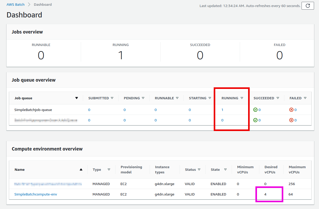
Pay attention to the part circled in red in Figure 65.
When a job is submitted, it goes through the state of SUBMITTED and then to the state of RUNNABLE.
RUNNABLE corresponds to the state of waiting for a new instance to be launched because there is not available instances in the compute environment to run the job.
When the instance is ready, the status of the job goes through STARTING to RUNNING.
Next, let’s look at the Desired vCPU of the compute environment when the status of the job is RUNNING (the part circled in purple in Figure 65).
The number 4 is the number of vCPU for one instance of g4dn.xlarge.
You can see that the minimum number of EC2 instances required to run the job has been launched in response to the job submission.
(If you are interested, you can also take a look at the EC2 console at the same time).
After a while, the status of the job will change from RUNNING to SUCCEEDED (or FAILED if an error occurs for some reason).
The training of MNIST used in this hands-on should take about 10 minutes.
Let’s wait until the job status becomes SUCCEEDED.
When the job completes, the training results (a CSV file containing the loss and accuracy for each epoch) will be saved in S3. You can check this from the AWS console.
If you go to the S3 console, you should find a bucket named simplebatch-bucketXXXX (the XXXX part depends on the user).
If you click on it and look at the contents, you will find a CSV file named metrics_lr0.0100_m0.1000.csv (Figure 66).
This is the result of training with learning rate = 0.01 and momentum = 0.1.
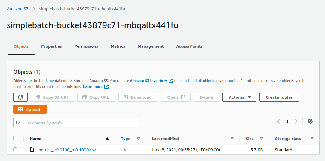
Now, let’s come back to run_single.ipynb.
In cells [5] through [7], we are downloading the CSV file of the training results.
 1
 2
 3
 4
 5
 6
 7
 8
 9
10
11
12
13
14
15
16
17
18
19
20
21
22
23
24
25
# [5]
import pandas as pd
import io
from matplotlib import pyplot as plt

# [6]
def read_table_from_s3(bucket_name, key, profile_name=None):
    if profile_name is None:
        session = boto3.Session()
    else:
        session = boto3.Session(profile_name=profile_name)
    s3 = session.resource("s3")
    bucket = s3.Bucket(bucket_name)

    obj = bucket.Object(key).get().get("Body")
    df = pd.read_csv(obj)

    return df

# [7]
bucket_name = "simplebatch-bucket43879c71-mbqaltx441fu"
df = read_table_from_s3(
    bucket_name,
    "metrics_lr0.0100_m0.1000.csv"
)
In [6], we define a function to download CSV data from S3 and load it as a pandas DataFrame object.
Note that when you run [7], you should replace the value of the bucket_name variable with the name of your own bucket.
(This is the simplebatch-bucketXXXX that we just checked from the S3 console).
Next, in cell [9], we plot the CSV data (Figure 67). We have successfully trained the MNIST model using AWS Batch, just as we did when we ran it locally!
 1
 2
 3
 4
 5
 6
 7
 8
 9
10
11
12
13
14
15
16
17
18
# [9]
fig, (ax1, ax2) = plt.subplots(1,2, figsize=(9,4))
x = [i for i in range(df.shape[0])]
ax1.plot(x, df["train_loss"], label="Train")
ax1.plot(x, df["val_loss"], label="Val")
ax2.plot(x, df["val_accuracy"])

ax1.set_xlabel("Epochs")
ax1.set_ylabel("Loss")
ax1.legend()

ax2.set_xlabel("Epochs")
ax2.set_ylabel("Accuracy")

print("Best loss:", df["val_loss"].min())
print("Best loss epoch:", df["val_loss"].argmin())
print("Best accuracy:", df["val_accuracy"].max())
print("Best accuracy epoch:", df["val_accuracy"].argmax())
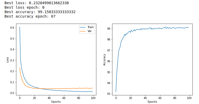
9.9. Submitting parallel jobs
Now, here comes the final part. Let’s use the AWS Batch system that we have built to perform real hyperparameter search.
Open the file run_sweep.ipynb in the same directory as run_single.ipynb that we just ran.
Cells [1], [2] and [3] are identical to run_single.ipynb.
 1
 2
 3
 4
 5
 6
 7
 8
 9
10
# [1]
import boto3
import argparse

# [2]
# AWS authentication helper. Skipping...

# [3]
def submit_job(lr:float, momentum:float, epochs:int, profile_name=None):
    # ...skip...
A for loop in cell [4] is used to prepare a grid of hyperparameter combinations and submit the jobs to the batch. In this case, 3x3=9 jobs are created.
1
2
3
4
# [4]
for lr in [0.1, 0.01, 0.001]:
    for m in [0.5, 0.1, 0.05]:
        submit_job(lr, m, 100)
After executing the cell [4], open the Batch console.
As before, you will see that the status of the jobs changes from SUBMITTED > RUNNABLE > STARTING > RUNNING.
Finally, make sure that all 9 jobs are in the RUNNING state (Figure 68).
Also, make sure that the Desired vCPUs of the compute environment is 4x9=36 (Figure 68).
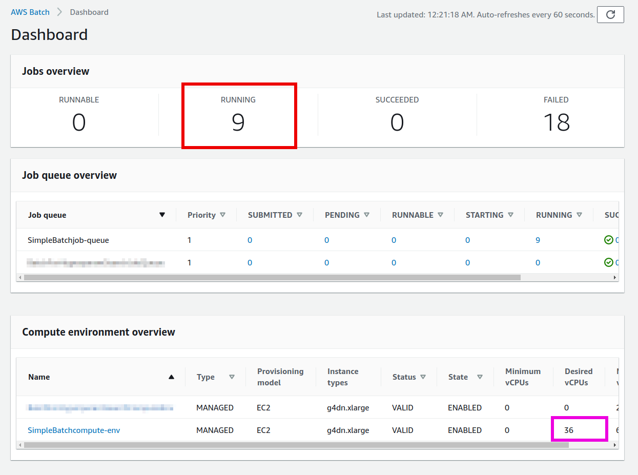
Next, let’s click Jobs from the left menu of the Batch console.
Here, you can see the list of running jobs (Figure 69).
It is also possible to filter jobs by their status.
You can see that all 9 jobs are in the RUNNING status.
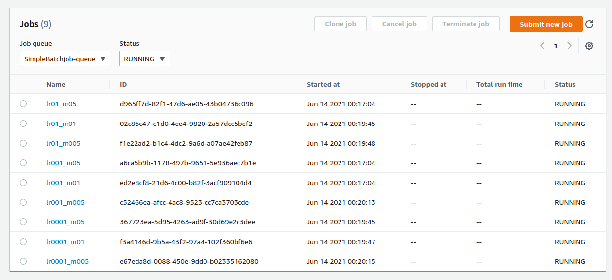
Now let’s take a look at the EC2 console.
Select Instances from the menu on the left, and you will see a list of running instances as shown in Figure 70.
You can see that 9 instances of g4dn.xlarge are running.
Batch has launched the necessary number of instances according to the job submission!
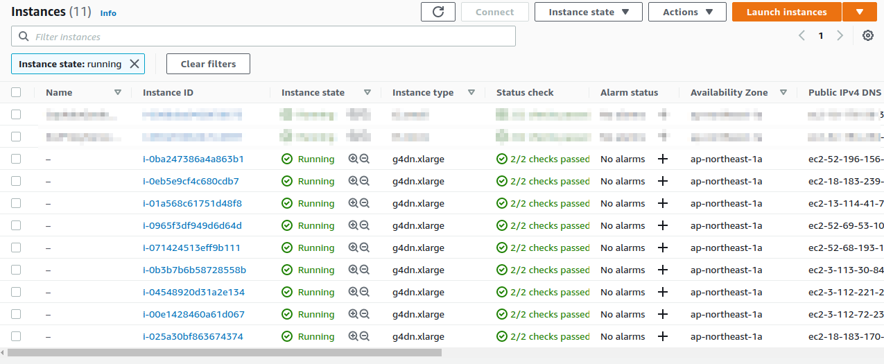
Once you have confirmed this, wait for a while until all jobs are finished (it takes about 10-15 minutes).
When all the jobs are finished, you should see the number of SUCCEEDED jobs on the dashboard is 9.
Also, make sure that the Desired vCPUs in the Compute environment has dropped to 0.
Finally, go to the EC2 console and check that all GPU instances are stopped.
In summary, by using AWS Batch, we were able to observe a sequence of events in which EC2 instances are automatically launched in response to job submissions, and the instances are immediately stopped upon completion of the job. Since it takes about 10 minutes to complete a single job, it would take 90 minutes if 9 hyperparameter pairs were calculated sequentially. By using AWS Batch to run these computations in parallel, we were able to complete all the computations in 10 minutes!
Let’s come back to run_sweep.ipynb.
In the cells after [5], the results of grid search are visualized.
 1
 2
 3
 4
 5
 6
 7
 8
 9
10
11
12
13
14
15
16
17
18
19
20
21
22
23
24
25
26
27
28
29
30
31
32
33
34
35
36
37
38
# [5]
import pandas as pd
import numpy as np
import io
from matplotlib import pyplot as plt

# [6]
def read_table_from_s3(bucket_name, key, profile_name=None):
    if profile_name is None:
        session = boto3.Session()
    else:
        session = boto3.Session(profile_name=profile_name)
    s3 = session.resource("s3")
    bucket = s3.Bucket(bucket_name)

    obj = bucket.Object(key).get().get("Body")
    df = pd.read_csv(obj)

    return df

# [7]
grid = np.zeros((3,3))
for (i, lr) in enumerate([0.1, 0.01, 0.001]):
    for (j, m) in enumerate([0.5, 0.1, 0.05]):
        key = f"metrics_lr{lr:0.4f}_m{m:0.4f}.csv"
        df = read_table_from_s3("simplebatch-bucket43879c71-mbqaltx441fu", key)
        grid[i,j] = df["val_accuracy"].max()

# [8]
fig, ax = plt.subplots(figsize=(6,6))
ax.set_aspect('equal')

c = ax.pcolor(grid, edgecolors='w', linewidths=2)

for i in range(3):
    for j in range(3):
        text = ax.text(j+0.5, i+0.5, f"{grid[i, j]:0.1f}",
                       ha="center", va="center", color="w")
The resulting plot is Figure 71.
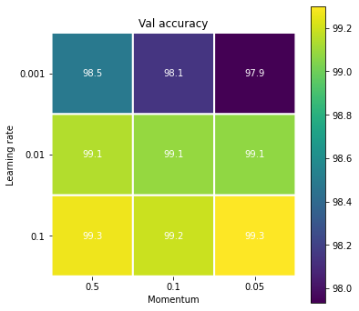
From this plot, we can see that the accuracy is maximum when the learning rate is 0.1, although the difference is small. It can also be seen that when the learning rate is 0.1, there is no significant performance gains between different momentum values.
|
It should be noted that this parameter search is extremely simplified for learning purposes. For example, in the experiment here the best learning rate turned out to be 0.1. However, this may be because the number of training epochs is limited to 100. The lower the learning rate, the more epochs are needed for training. If the number of training epochs is increased, different results may be observed. In this study, we used 48,000 of the 60,000 training data from MNIST as training data and the remaining 12,000 as validation data. However, if you are concerned about the bias of the data due to the split, you may want to evaluate the model multiple times by changing the split (k-fold cross-validation) as a more sophisticated approach. |
In this hands-on session, we experienced the steps to optimize the hyperparameters of the MNIST classification model. By using AWS Batch, we were able to build a system that can dynamically control EC2 clusters and process jobs in parallel. If you can master EC2 to this level, you will be able to solve many problems on our own!
9.10. Deleting the stack
This concludes the hands-on session.
Finally, let’s delete the stack.
In order to delete the stack for this hands-on, the Docker images placed in the ECR must be deleted manually.
If you don’t do this, you’ll get an error when you run cdk destroy.
This is a CloudFormation specification that you have to follow.
To delete a Docker image in ECR, go to the ECR console and open the repository where the image is located.
Then, click the DELETE button on the upper right corner of the screen to delete it (Figure 72).
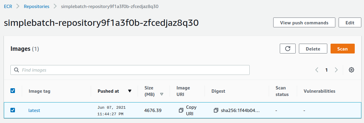
Alternatively, to perform the same operation from the AWS CLI, use the following command (replace XXXX with the name of your ECR repository).
$ aws ecr batch-delete-image --repository-name XXXX --image-ids imageTag=latestAfter the image has been deleted, use the following command to delete the stack.
$ cdk destroy[sec:batch_development_and_debug] === Development and debugging of machine learning applications using the cloud
In the hands-on session described in this chapter, we used AWS Batch to run parallel neural network trainings to accelerate the model development. As the last topic in this chapter, we will discuss how to develop and debug machine learning applications using the cloud.
If you don’t have a powerful local machine with GPUs, and you have the budget to use the cloud, then a development scheme like Figure 73 would be ideal.
In the first stage, create an EC2 instance with GPUa using the method described in Section 6, and experiment with various models in an interactive environment such as Jupyter Notebook.
When the application is completed to some extent with Jupyter, package the application into a Docker image.
Then, run docker run on EC2 to check if the created image works without errors.
Next, we will perform tuning, such as hyperparameter optimization, using a computational system such as AWS Batch, which we learned in the Section 9.
Once we have a good deep learning model, we will build a system to perform inference on large-scale data, using Section 8 as a reference.
In fact, the exercises in this book have been carried out along this workflow. We first experimented with a model for solving the MNIST task using Jupyter Notebook, then packaged the code into Docker, and used AWS Batch to perform a hyperparameter search. By repeating this cycle, we can proceed with the development of machine learning applications that take full advantage of the cloud.
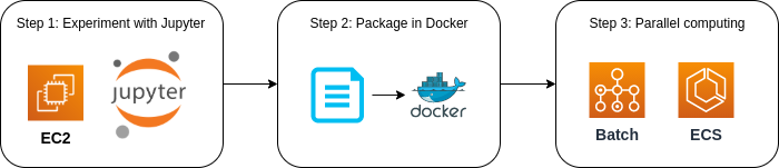
9.11. Short summary
This concludes Part II of this book. We hope you enjoyed the journey exploring the cloud technology.
In Part II, we first explained how to launch an EC2 instance with GPUs in order to run deep learning calculations in the cloud. In the hands-on session, we trained a neural network to solve the MNIST digit recognition task using a virtual server launched in the cloud (Section 6).
We also explained the steps to create a cluster using Docker and ECS as a means to build large scale machine learning applications (Section 7). As an exercise, we deployed a bot in the cloud that automatically generates answers to text questions given in English (Section 8). You should have been able to get some experience how computational resources are created and deleted dynamically in response to the submission of tasks.
Furthermore, in Section 9, we introduced a method to train neural networks in parallel using AWS Batch. Although the methods introduced here are minimal, they cover the essence of how to scale up a computer system. We hope that these hands-on experiences have given you some idea of how to apply cloud technology to solve real-world problems.
In the third part of this book, we take it a step further and explain the latest cloud design method called serverless architecture. In the hands-on session, we will implement a simple SNS service from scratch. Let’s continue our journey to enjoy the cutting-edge frontiers of cloud computing!
10. How to create web services
This is the third part of the book. In the previous sections, we have explained how to start a virtual server in the cloud and run computations on it. Using EC2, ECS, Fargate, and Batch, we have configured dynamically scaling clusters and implemented cloud systems that execute tasks in parallel. In retrospect, you may notice that the techniques we have introduced so far have been focused on embracing the cloud to solve your own scientific or engineering problem. On the other hand, another important role of the cloud is to provide computing services and databases that can be used by the general public.
In Part III, which begins with this section, we would like to take a slightly different direction from the previous lectures and discuss how to deploy applications on the cloud and make them widely available to the general public. Through this lecture, we will learn how web services in the real world are created, and how to build such applications from scratch. In the process, we will explain the latest cloud design method called serverless architecture.
As a prelude, this chapter provides an overview of the technology behind the web services and introduces some concepts and terminology. Theyse are essential knowledge for the hands-on exercises that follow, so please take your time to understand them well.
10.1. How Web Services Work — Using Twitter as an Example
When you access Twitter, Facebook, YouTube, and other web services from your computer or smartphone, what is actually happening to render the contents in the page?
Many readers may already be familiar with the communication between servers and clients via HTTP, and since it would take up too much space to thoroughly explain everything, we will only cover the essentials here. In the following, we will use Twitter as a concrete example to outline the communication between the server and the client. As a sketch, Figure 74 depicts the communication between the client and the server.
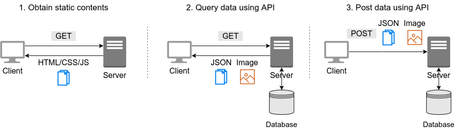
As a premise, the client-server communication is done using HTTP (Hypertext Transfer Protocol). Recently, it has become a standard to use HTTPS (Hypertext Transfer Protocol Secure), which is an encrypted HTTP. In the first step, the client obtains static content from the server through HTTP(S) communication. Static content includes the main body of a web page document written in HTML (Hypertext Markup Language), page design and layout files written in CSS (Cascading Style Sheets), and programs that define the dynamic behavior of the page written in JavaScript (JS). In the design of modern web applications, including Twitter, these static files only define the "frame" of the page, and the content (e.g., the list of tweets) must be retrieved using API (Application Programming Interface). Therefore, the client sends the API request to the server according to the program defined in the JavaScript, and obtains the tweet list. JSON (JavaScript Object Notation) is often used to exchange text data. Media content such as images and videos are also retrieved by the API in the same way. The text and images retrieved in this way are embedded in the HTML document to create the final page presented to the user. Also, when posting a new tweet, the client uses the API to write the data to the server’s database.
10.2. REST API
API (Application Programming Interface) is a term that has been frequently used in this book, but we will give a more formal definition here. An API is a general term for an interface through which an application can exchange commands and data with external software. Especially in the context of web services, it refers to the list of commands that a server exposes to the outside world. The client obtains the desired data or sends data to the server by choosing the appropriate API commands.
Especially in the context of the web, APIs based on a design philosophy called REST (Representational State Transfer) are most commonly used. An API that follows the REST design guidelines is called a REST API or RESTful API.
A REST API consists of a pair of Method and URI (Universal Resource Identifier), as shown in Figure 75.
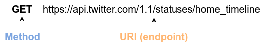
A method can be thought of as a "verb" that abstractly expresses the kind of desired operation.
Methods can use any of the nine verbs defined in the HTTP standard.
Among them, the five most frequently used ones are GET, POST, PUT, PATCH, and DELETE (Table 6).
The operations using these five methods are collectively called CRUD (create, read, update, and delete).
| Method | Intended behaviour |
|---|---|
GET |
Obtaining items |
POST |
Creating a new item |
PUT |
Replacing an existing item with a new one |
PATCH |
Updating a part of an existing item |
DELETE |
Deleting an item |
On the other hand, a URI represents the target of an operation, i.e., the "object".
In the context of the web, the target of an operation is often referred to as a resource.
The URI often begins with the address of the web server, starting with http or https, and the path to the desired resource is specified after the / (slash).
In the example of Figure 75, it means to retrieve (GET) the resource /1.1/status/home_timeline with the address https://api.twitter.com.
(Note that the number 1.1 here indicates the API version.)
This API request retrieves the list of tweets in the user’s home timeline.
|
In addition to the methods listed in Table 6, other methods defined in the HTTP protocol (OPTIONS, TRACE, etc.) can be used for the REST API methods, but they are not so common. In some cases, these methods alone are not enough to express a verb, but the meaning may be made clearer by using explicit path in URI.
For example, the Twitter API for deleting tweets is defined as |
|
The concept of REST was established in the early 2000s and has become the standard for API design today. As web technology advances, on the other hand, the demand for new API design is growing. One approach that has become particularly popular in recent years is GraphQL.s GraphQL was first created by Facebook, and is currently maintained and updated by the GraghQL Foundation. GraphQL has several advantages over REST, including the ability for clients to query data with greater flexibility. |
10.3. Twitter API
In order to have a more realistic feeling on the web APIs, let’s take a look at Twitter’s API. A list of APIs provided by Twitter can be found at Twitter’s Developer Documentation. Some representative API endpoints are listed in Table 7.
| Endpoint | Expected behaviour |
|---|---|
|
Get the list of tweets in the home timeline. |
|
Get the details of the tweet specified by |
|
Search for tweets |
|
Post a new tweet |
|
Upload images |
|
Delete a tweet specified by |
|
Retweet a tweet specified by |
|
Undo retweet of a tweet specified by |
|
Like the selected tweet. |
|
Undo like of the selected tweet. |
Based on this list of APIs, let’s simulate the client-server communication that happens when you open a Twitter app or website.
When a user opens Twitter, the first API request sent to the server is GET statuses/home_timeline, which retrieves a list of tweets in the user’s home timeline.
Each tweet is in JSON format and contains attributes such as id, text, user, coordinates, and entities.
The id represents the unique ID of the tweet, and the text contains the body of the tweet.
The user is a JSON data containing the information of the user who posted the tweet, including the name and URL of the profile image.
The coordinates contains the geographic coordinates of where the tweet was posted.
entities contains the links to media files (images, etc.) related to the tweet.
From GET statuses/home_timeline, a list of the most recent tweets is retrieved (or a part of the list if the list is too long).
If you know the ID of the tweet, you can call GET statuses/show/:id to retrieve the specific tweet specified by the :id parameter.
The GET search API is used to search tweets.
The GET search API can be used to search for tweets by passing various query conditions, such as words in the tweet, hashtags, and the date, time, and location of the tweet.
The API will return the tweet data in JSON format, similar to GET statuses/home_timeline.
When a user posts a new tweet, the POST statuses/update endpoint is used.
The POST statuses/update endpoint receives the text of the tweet, and in the case of a reply, the ID of the tweet to which the user is replying.
If you want to attach images to the tweet, use POST media/upload as well.
To delete a tweet, POST statuses/destroy/:id is used.
Other frequently used operations are POST statuses/retweet/:id and POST statuses/unretweet/:id.
These APIs are used to retweet or unretweet the tweet specified by :id, respectively.
In addition, POST favorites/create and POST favorites/destroy can be used to add or remove a "like" to a selected tweet.
This is the sequence of operations that takes place behind Twitter applications. If you want to create your own bot, you can do so by writing a custom program that combines these APIs.
As you can see, APIs are the most fundamental element in the construction of any web service. In the following sections, the terms introduced in this section will appear many times, so please keep them in mind before reading on.
11. Serverless architecture
Serverless architecture or serverless computing is a way of designing cloud systems based on a completely different approach. Historically, Lamba, released by AWS in 2014, is considered as a pioneer of serverless architecture. Since then, other cloud platforms such as Google and Microsoft have started to provide similar features. The advantage of serverless architecture is that it enables the creation of scalable cloud systems inexpensively and easily, and it is rapidly being adopted by many cloud systems in recent years.
Serverless literally means computing without servers, but what does it actually mean? In order to explain serverless, we must first explain the traditional "serverful" system.
11.1. Serverful cloud (conventional cloud)
A sketch of a traditional cloud system is shown in Figure 76. The request sent from the client is first sent to the API server. In the API server, tasks are executed according to the content of the request. Some tasks can be completed by the API server alone, but in most cases, reading and writing of the database is required. In general, an independent server machine dedicated to the database is used. Large sized data, such as images and videos, are often stored on a separate storage server. These API servers, database servers, and storage servers are all independent server machines. In AWS terms, you can think of them as virtual instances of EC2.
Many web services are designed to have multiple server machines running in the cloud to handle requests from a large number of clients. The operation of distributing requests from clients to servers with enough computing capacity is called load balancing, and the machine in charge of such operation is called load balancer.
Launching a large number of instances for the purpose of distributing the computational load is fine, but it is a waste of cost and power if the computational load is too small and the most of the cluster is kept idling. Therefore, we need a mechanism that dynamically increases or decreases the number of virtual servers in a cluster according to the computational load so that all servers always maintain the certain load. Such a mechanism is called cluster scaling, and the operation of adding a new virtual instance to the cluster in response to an increase in load is called scale-out, and the operation of shutting down an instance in response to a decrease in load is called scale-in. Scaling of clusters is necessary not only for API servers, but also for database servers and storage servers. In the storage server, for example, frequently accessed data is stored in the cache area, and multiple copies of the data are made across instances. In the same way, database servers require distributed processing to prevent frequent data accesses from disrupting the system. It is necessary to adjust the load so that it is evenly distributed throughout the cloud system, and developers must spend a lot of time tuning the system. In addition, the scaling settings need to be constantly reviewed according to the number of users of the service, and continuous development is required.
What makes the matters worse, the tasks processed by the API server are non-uniform. Being non-uniform, means that, for example, task A consumes 3000 milliseconds of execution time and 512MB of memory, while another task B consumes 1000 milliseconds of execution time and 128MB of memory. Scaling a cluster becomes complex when a single server machine handles multiple tasks with different computational loads. In order to simplify this situation, it is possible to design the cluster so that only one type of task is executed by a single server, but there are many negative effects of adopting such design.
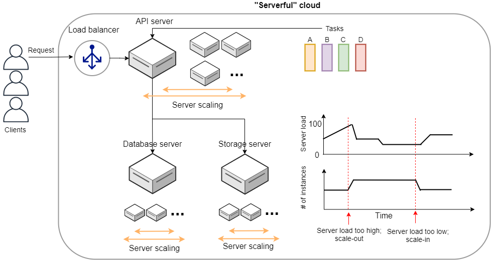
11.2. To the serverless cloud
As we discussed in Section 11.1, scaling of clusters is an essential task to maximize the economic efficiency and system stability of cloud systems. Reflecting this, a lot of developer’s time and efforts have been invested in it.
Scaling a cluster is a task that all developers have done over and over again, and if some aspects could be templated and made common, it would greatly reduce the cost of development. In order to achieve this, one needs to rethink the design of cloud systems from a fundamental level. Is there a cloud system design that is simpler and more efficient by considering scaling as a first and built-in priority? Such was the motivation behind the birth of serverless architecture.
The biggest problem with conventional serverful systems is that users occupy the entire server. Namely, when an EC2 instance is launched, it is available only to the user who launched it, and the computation resources (CPU and RAM) are allocated exclusively to that user. Since a fixed allocation of computing resources has been made, the same cost will be incurred in proportion to the launch time, regardless of whether the instance’s computing load is 0% or 100%.
The starting point of serverless architecture is the complete elimination of such exclusively allocated computational resources. In a serverless architecture, all computation resources are managed by the cloud provider. Rather than renting an entire virtual instance, clients submit a program or commands to the cloud every time they need to perform a computational task. The cloud provider tries to find free space from its own huge computational resources, executes the submitted program, and returns the execution result back to the client. In other words, the cloud provider takes care of the scaling and allocation of computational resources, and the user focuses on submitting jobs. This can be illustrated as Figure 77.
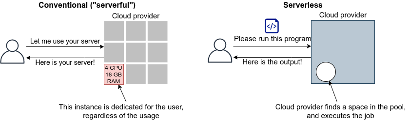
In a serverless cloud, scalability is guaranteed because all scaling is taken care of by the cloud provider. Even if a client sends a large number of tasks at the same time, the cloud provider’s sophisticated system ensures that all tasks are executed without delay. Also, by using a serverless cloud, the cost of the cloud is determined by the total amount of computation. This is a big difference compared to conventional systems where the cost is determined by the launch time of the instance regardless of the total amount of computation performed.
Since serverless cloud is a fundamentally different approach from traditional cloud, the way to design the system and write code is very different. To develop and operate a serverless cloud, it is necessary to be familiar with concepts and terminology specific to serverless technology.
|
Traditional cloud systems running many virtual instances may be analogous to renting a room. When you rent a room, the monthly rent is constant, regardless of how much time you spend in the room. Similarly, a virtual server incurs a fixed fee per hour, regardless of how much computation it is doing. On the other hand, serverless clouds are similar to electricity, water, and gas bills. In this case, the fee is determined in proportion to the amount actually used. The serverless cloud is also a system where the fee is determined by the total amount of time the calculation is actually performed. |
11.3. Components that make up a serverless cloud
Now that we have an overview of serverless architecture, let us introduce you to the components that make up a serverless cloud in AWS. In particular, we will focus on Lambda, S3, and DynamoDB (Figure 78). In a serverless cloud, a system is created by integrating these components. In what follows, we will go through all the knowledge that must be kept in mind when using Lambda, S3, and DynamoDB, so it may be difficult to get a concrete image. However, in the next section (Section 12), we will provide hands-on exercises for each of them, so you can deepen your understanding.
11.3.1. Lambda
The core of serverless computing in AWS is Lambda. The summary of Lambda is illustrated in Figure 79. The workflow with Lambda is simple. First, users register the code of the program they want to execute. Programs are supported in major languages such as Python, Node.js, and Ruby. Each program registered with Lambda is referred to as a function. When a function is to be executed, an invoke command is sent to Lambda. As soon as Lambda receives the invoke request, it starts executing the program, within a few milliseconds to a few hundred milliseconds latency. It then returns the execution results to the client or other programs.
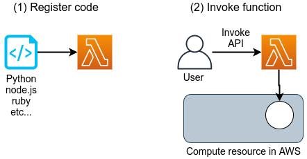
As you can see, in Lambda, there is no occupied virtual instance, only a program waiting to be executed. In response to an invoke request, the program is placed somewhere in the huge AWS compute pool and executed. Even if multiple requests come in at the same time, AWS allocates computing resources to execute them, and processes them in parallel. In principle, Lambda is able to execute thousands or tens of thousands of requests at the same time. This kind of service that dynamically executes functions without the existence of an occupied virtual server is collectively called FaaS (Function as a Service).
Lambda can use 128MB to 10240MB of memory for each function (specifications at the time of writing).
The effective CPU power is allocated in proportion to the amount of memory.
In other words, the more memory allocated to a task, the more CPU resources will be allocated to it.
(However, AWS does not provide a specific conversion table for RAM and CPU power.)
The execution time is recorded in units of 100 milliseconds, and the price is proportional to the execution time.
Table 8 is the Lambda pricing table (when ap-north-east1 region is selected at the time of writing).
| Memory (MB) | Price per 100ms |
|---|---|
128 |
$0.0000002083 |
512 |
$0.0000008333 |
1024 |
$0.0000016667 |
3008 |
$0.0000048958 |
In addition to the fee proportional to the execution time, there is a fee for each request sent. This is $0.2 per million requests. For example, if a function that uses 128MB of memory is executed 200 milliseconds each, for a total of 1 million times, then the total cost would be 0.0000002083 * 2 * 10^6 + 0.2 = $0.6. Since many functions can be executed in about 200 milliseconds for simple calculations such as updating the database, the cost is only $0.6 even if the database is updated one million times. In addition, if the code is in a waiting state without being executed, the cost is zero. In this way, cost will be chaged for only the time when meaningful processing is performed.
Lambda is most suitable for executing highly repetitive tasks that can be completed in a relatively short time. Reading and writing databases is a typical example, but other possible uses include cropping the size of an image or performing periodic server-side maintenance. It is also possible to connect multiple Lambdas in a relay fashion, and complex logic can be expressed by combining simple processes.
|
It should be noted that the Lambda fee calculation described above omits some factors that contribute to the cost for the sake of explanation. For example, it does not take into account the cost of reading and writing DynamoDB or the cost of network communication. |
11.3.2. Serverless storage: S3
The concept of serverless has been extended to storage as well.
Conventional storage (file system) requires the presence of a host machine and an OS. Therefore, a certain amount of CPU resources must be allocated, even if it does not require much power. In addition, with conventional file systems, the size of the storage space must be determined when the disk is first initialized, and it is often difficult to increase the capacity later. (Using a file system such as ZFS, it is possible to change the size of the file system freely to some extent.) Therefore, in traditional cloud computing, you have to specify the size of the disk in advance when you rent a storage space, and you will be charged the same fee whether the disk is empty or full (Figure 80).
Simple Storage Service (S3) provides a serverless storage system (Figure 80). Unlike conventional storage systems, S3 does not have the concept of being "mounted" on the OS. Basically, data read/write operations are performed through APIs. In addition, operations that normally require the intervention of the OS and CPU, such as data redundancy, encryption, and backup creation, can also be performed through the API. With S3, there is no predetermined disk space size, and the total storage space increases as more data is stored in S3. In principle, it is possible to store petabyte-scale data. The price of storage is determined by the total amount of the data stored.
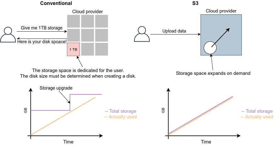
Table 9 summarizes the main factors related to pricing when using S3.
(This is for the us-east-1 region.
Only the major points are taken out for the sake of explanation.
For details, see
Official Documentation "Amazon S3 pricing"]).
| Item | Price |
|---|---|
Data storage (First 50TB) |
$0.023 per GB per month |
PUT, COPY, POST, LIST requests (per 1,000 requests) |
$0.005 |
GET, SELECT, and all other requests (per 1,000 requests) |
$0.0004 |
Data Transfer IN To Amazon S3 From Internet |
$0 |
Data Transfer OUT From Amazon S3 To Internet |
$0.09 per GB |
First, data storage costs $0.025 per GB per month.
Therefore, if you store 1000GB of data in S3 for a month, you will be charged $25.
In addition, requests such as PUT, COPY, and POST (i.e., operations to write data) incur a cost of $0.005 per 1000 requests, regardless of the amount of data.
Requests such as GET and SELECT (= operations to read data) incur a cost of $0.0004 per 1000 requests.
S3 also incurs a cost for communication when retrieving data out of S3.
At the time of writing, transferring data from S3 to the outside via the Internet (data-out) incurs a cost of $0.09 per GB.
Sending data into S3 via the Internet (data-in) is free of charge.
Transferring data to services in the same AWS region (Lambda, EC2, etc.) is also free.
There is a cost for transferring data across AWS regions.
In any case, in keeping with the serverless concept, all fees are determined on a pay-as-you-go basis.
11.3.3. Serverless database: DynamoDB
The concept of serverless can also be applied to databases. A database here refers to a fast storage area for web services to record data such as user and product information. Some of the popular databases include MySQL, PostgreSQL, MongoDB.
The difference between a database and ordinary storage is in the data retrieval function. In ordinary storage, data is simply written to disk. In a database, data is arranged in a way that makes searching more efficient, and frequently accessed data is cached in memory. This makes it possible to retrieve the elements of interest from a huge amount of data rapidly.
Naturally, the involvement of a CPU is essential to realize such a search function. Therefore, when constructing a conventional database, a machine with a large number of CPU cores is often used in addition to the large storage space. Often, a distributed system consisted of multiple machines is designed to host a massive database. In the case of a distributed system, it is necessary to scale appropriately according to the access load to the database, as discussed in Section 11.1.
DynamoDB is a serverless and distributed database provided by AWS. Because it is serverless, there is no occupied virtual instance for the database, and operations such as writing, reading, and searching data are performed through APIs. As with S3, there is no upper limit to the data storage space, and the storage space increases as more data is stored. In addition, DynamoDB automatically handles scaling when the load on the database increases or decreases, eliminating complicated programming to control the database scaling.
The calculation of DynamoDB pricing is rather complicated, but Table 10 summarizes the main factors involved in pricing when using the "On-demand Capacity" mode.
(The table is for the us-east-1 region.
For details, see
Official Documentation "Pricing for On-Demand Capacity").
| Item | Price |
|---|---|
Write request units |
$1.25 per million write request units |
Read request units |
$0.25 per million read request units |
Data storage |
$0.25 per GB-month |
In DynamoDB, the unit for data write operations is called a write request unit, and the unit for data read operations is called a read request unit. Basically, writing data of 1kB or less once consumes 1 write request unit, and reading data of 4kB or less once consumes 1 read request unit. (For details, see Official Documentation "Read/Write Capacity Mode"). The cost of write request units is set at $1.25 per million requests, and the cost of read request units is set at $0.25 per million requests. There is also a monthly cost of $0.25 per GB chaged for stored data. Since DynamoDB is a database with a high-speed search function, the storage cost per GB is about 10 times higher than S3. The cost of DynamoDB data transfer is zero for both data-in and data-out within the same region. A separate cost is incurred for communication across regions.
11.3.4. Other serverless components in AWS
Lambda, S3, and DynamoDB described above are the most frequently used services in serverless cloud. Other components of serverless cloud are listed below. Some of them will be explained during the hands-on sessions in the later sections.
-
API Gateway: This is responsible for routing when building the REST API. It will be covered in Section 13.
-
Fargate: Fargate, which we used in Section 8, is another element of the serverless cloud. The difference between Fargate and Lambda is that Fargate can perform calculations that require a larger amount of memory and CPU than Lambda.
-
Simple Notification Service (SNS): A service for exchanging events between serverless services.
-
Step Functions: Orchestration between serverless services.
|
Is serverless architecture a solution for everything? We think the answer to this question is no. Serveless is still a new technology, and it has several disadvantages or limitations compared to serverful system. One major disadvantage is that serverless systems are specific to each cloud platform, so they can only be operated on a particular platform. Migrating a serverless system created in AWS to Google’s cloud, for example, would require a rather large rewrite of the program. On the other hand, for serverful systems, migration between platforms is relatively easy. This is probably the cloud providers' buisiness strategy to increase the dependency on their own systems and keep their customers. Other limitations and future challenges of serverless computing are discussed in detail in the following paper. |
12. Hands-on #5: Introduction to serverless computing
In the previous chapter, we gave an overview of serverless architecture. In this chapter, let’s learn how to use serverless cloud through hands-on exercises. In this hands-on session, we will go through three serverless cloud components: Lambda, S3, and DynamoDB. A short tutorial is provided for each of them.
12.1. Lambda hands-on
First, let’s learn how to use Lambda. The source code for the hands-on is available on GitHub at handson/serverless/lambda.
A sketch of the application used in this hands-on is shown in Figure 81. In STEP 1, code written in Python is registered to Lambda using AWS CDK. Then, in STEP 2, we use the invoke API to launch multiple Lambdas simultaneously to perform parallel computations. This is a minimal setup for the purpose of experiencing the Lambda workflow.
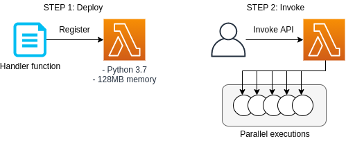
|
This hands-on exercise can be performed within the free Lambda tier. |
The program to deploy is written in app.py. Let’s take a look at the code.
 1
 2
 3
 4
 5
 6
 7
 8
 9
10
11
12
13
14
15
16
17
18
19
20
21
22
23
24
25
26
27
(1)
FUNC = """
import time
from random import choice, randint
def handler(event, context):
    time.sleep(randint(2,5))
    sushi = ["salmon", "tuna", "squid"]
    message = "Welcome to Cloud Sushi. Your order is " + choice(sushi)
    print(message)
    return message
"""

class SimpleLambda(Stack):

    def __init__(self, scope: Construct, construct_id: str, **kwargs) -> None:
        super().__init__(scope, construct_id, **kwargs)

        (2)
        handler = _lambda.Function(
            self, 'LambdaHandler',
            runtime=_lambda.Runtime.PYTHON_3_7,
            code=_lambda.Code.from_inline(FUNC),
            handler="index.handler",
            memory_size=128,
            timeout=cdk.Duration.seconds(10),
            dead_letter_queue_enabled=True,
        )
| 1 | Here, we define a function that should be executed by Lambda. This is a very simple function that sleeps for a random period of 2-5 seconds, then randomly selects one of the strings ["salmon", "tuna", "squid"], and returns a message "Welcome to Cloud Sushi. Your order is XXXX" (where XXXX is the chosen sushi item). |
| 2 | Next, the function written in <1> is registered in Lambda.
The meanings of the parameters are quite obvious, but let us explin for the completeness.
|
By running the above program, a Lambda function will be created in the cloud. Now let’s deploy it.
12.1.1. Deploying the application
The deployment procedure is almost the same as the previous hands-on.
Here, only the commands are listed (lines starting with # are comments).
If you have forgotten the meaning of each command, review the first hands-on.
You should not forget to set the access key (Section 14.3).
# move to the project directory
$ cd handson/serverless/lambda

# create venv and install dependent libraries
$ python3 -m venv .env
$ source .env/bin/activate
$ pip install -r requirements.txt

# deploy!
$ cdk deploy
If the deployment command is executed successfully, you should get an output like Figure 82.
In the output you should see a message FunctionName = SimpleLambda-XXXX where XXXX is some random string.
We will use this XXXX string later, so make a note of it.
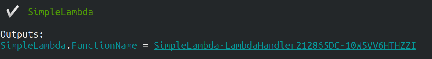
cdk deployLet’s log in to the AWS console and check the deployed stack. If you go to the Lambda page from the console, you can see the list of Lambda functions (Figure 83).
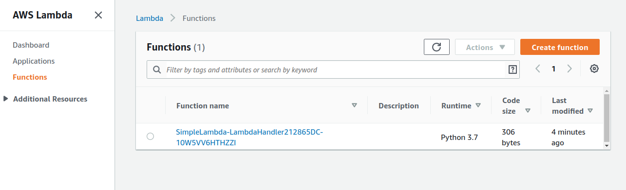
In this application, we have created a function with a name SimpleLambda-XXXX.
Click on the name of the function to see the details.
You should see a screen like Figure 84.
In the editor, you can see the Python function that you have just defined in the code.
Scroll down to the bottom of the screen to see the various settings for the function.
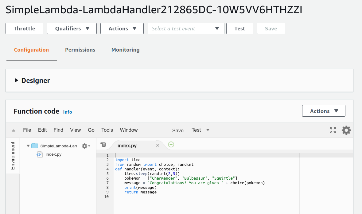
|
The code executed by Lambda can also be edited using the editor on the Lambda console screen (Figure 84). In some cases, it is faster to directly edit the code here for debugging purpose. In this case, do not forget to update the CDK code to reflect the edits you made. |
12.1.2. Executing Lambda function
Now, let’s execute (invoke) the Lambda function we have created. Using the AWS API, we can start executing the function. Here, we will use the handson/serverless/lambda/invoke _one.py, which contains a simple code to invoke Lambda function. Interested readers are recommended to read the code.
The following command invokes a Lambda function.
Replace the XXXX part of the command with the string obtained by SimpleLambda.FunctionName = SimpleLambda-XXXX when you deployed it earlier.
$ python invoke_one.py SimpleLambda-XXXXAfter a few seconds, you should get the output "Welcome to Cloud Sushi. Your order is salmon".
It seems like a toy example, but the function was indeed executed in the cloud, where it generated a random number, selected a random sushi item, and returned the output.
Try running this command a few times and see that different sushi menu is returned for each execution.
Now, this command executes one function at a time, but the real power of Lambda is that it can execute a large number of tasks at the same time. Next, let’s try sending 100 tasks at once. We use a Python script saved as handson/serverless/lambda/ invoke_many.py.
Run the following command.
Remember to replace the XXXX part as before.
The second argument, 100, means to submit 100 tasks.
$ python invoke_many.py XXXX 100The output will be something like below.
....................................................................................................
Submitted 100 tasks to Lambda!
Let’s confirm that 100 tasks are actually running simultaneously. Go back to the Lambda console (Figure 84), and click on the "Monitoring" tab. You will see a graph like Figure 85.
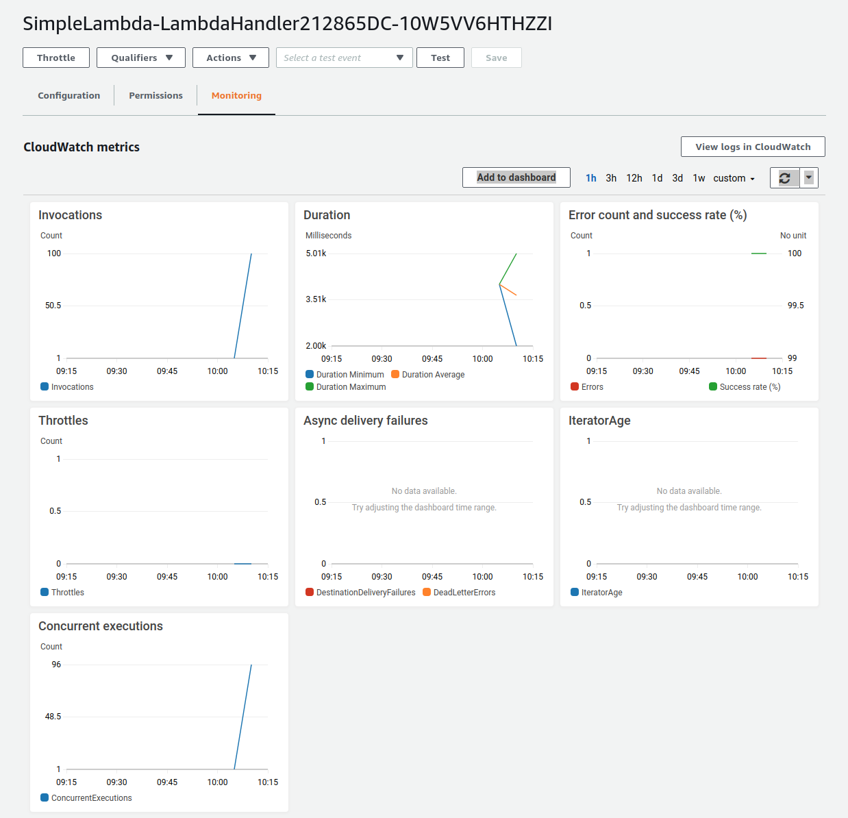
|
It takes some time for the graph shown in Figure 85 to be updated. If nothing is shown, wait a while and refresh the graph again. |
In Figure 85, "Invocations" means how many times the function has been executed. You can see that it has been indeed executed 100 times. Furthermore, "Concurrent executions" shows how many tasks were executed simultaneously. In this case, the number is 96, which means that 96 tasks were executed in parallel. (The reason this does not equal 100 is that the commands to start the tasks were not sent at exactly the same time.)
As we just saw, although it is very simple, using Lambda, we were able to create a cloud system that can execute a task concurrently.
If we tried to do this in a traditional serverful cloud, we would have to write a lot of code for scaling the cluster, and also adjust various parameters.
|
If you are interested, you can try submitting 1000 tasks at once. You will see that Lambda can handle such a large number of requests. However, be careful not to overdo it, or you will exceed the free usage limit of Lambda. |
12.1.3. Deleting the stack
Finally, let’s remove the stack. To remove the stack, execute the following command.
$ cdk destroy12.2. DynamoDB hands-on
Next, let’s work on a short tutorial on DynamoDB. The source code for the hands-on is available on GitHub at /handson/serverless/dynamodb.
A sketch of the application used in this hands-on is shown in Figure 86. In STEP 1, we deploy an empty DynamoDB tables using AWS CDK. Then, in STEP 2, we practice basic operations such as writing, reading, and deleting data from the database using the API.
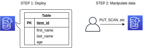
|
This hands-on exercise can be performed within the free DynamoDB tier. |
The program to deploy is written in handson/serverless/dynamodb/app.py. Let’s take a look at the code.
 1
 2
 3
 4
 5
 6
 7
 8
 9
10
11
12
13
14
15
16
class SimpleDynamoDb(Stack):
    def __init__(self, scope: Construct, construct_id: str, **kwargs) -> None:
        super().__init__(scope, construct_id, **kwargs)

        table = ddb.Table(
            self, "SimpleTable",
            (1)
            partition_key=ddb.Attribute(
                name="item_id",
                type=ddb.AttributeType.STRING
            ),
            (2)
            billing_mode=ddb.BillingMode.PAY_PER_REQUEST,
            (3)
            removal_policy=cdk.RemovalPolicy.DESTROY
        )
With this code, an empty DynamoDB table with the minimum configuration is created. Let us explain the meanings of each parameter.
| 1 | Here we define partition key of the table.
Every DynamoDB table must have a partition key.
The partition key is a unique ID for each element (record) in the table.
Every record in the table must have a partition key.
There cannot be more than one element with the same partition key in a table.
(except for the case where sort Key is used. For more information, see
official documentation "Core Components of Amazon DynamoDB").
In this example, the partition key is named item_id. |
| 2 | Here we specify the billing_mode parameter.
By specifying ddb.BillingMode.PAY_PER_REQUEST, DynamoDB table in on-demand capacity mode is created.
There is another mode called PROVISIONED, but this is for more advanced use cases. |
| 3 | Here we specify the removal_policy.
It specifies whether DynamoDB table will be removed together when the CloudFormation stack is deleted.
In this code, DESTROY is selected, so all the data will be deleted.
If you select other options, you can define other behaviors such as keeping DynamoDB backups even if the stack is deleted. |
12.2.1. Deploying the application
The deployment procedure is almost the same as the previous hands-on.
Here, only the commands are listed (lines starting with # are comments).
If you have forgotten the meaning of each command, review the first hands-on.
You should not forget to set the access key (Section 14.3).
# move to the project directory
$ cd handson/serverless/dynamodb

# create venv and install dependent libraries
$ python3 -m venv .env
$ source .env/bin/activate
$ pip install -r requirements.txt

# deploy!
$ cdk deploy
If the deployment command is executed successfully, you should get an output like Figure 87.
In the output you should see a message TableName = XXXX where XXXX is some random string.
We will use this XXXX string later, so make a note of it.
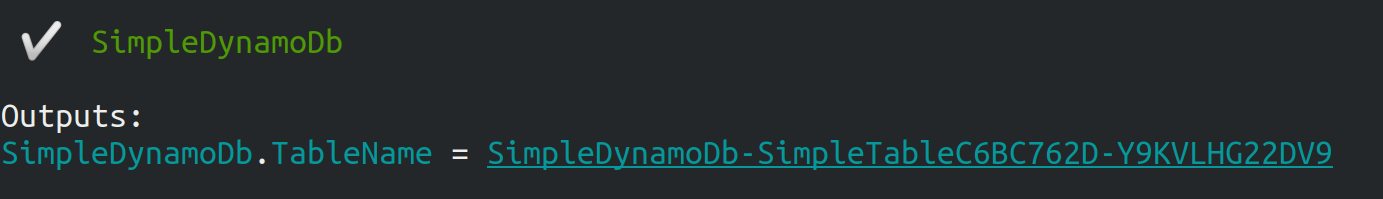
cdk deployLet’s log in to the AWS console and check the deployed stack. From the console, go to the DynamoDB page and select "Tables" from the menu bar on the left. Then, you can see the list of tables in a screen like Figure 88.
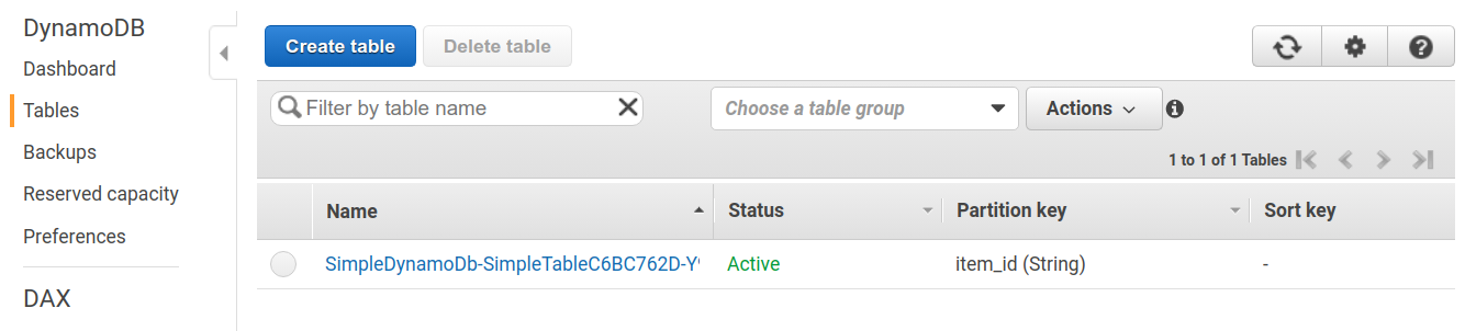
The deployment will createa a table with a random name starting with SimpleDynamoDb.
Click on the name of the table to see the details.
You should see a screen like Figure 89.
Click on the "Items" tab to see the records in the table.
At this point, the table is empty because no data has been written to it.
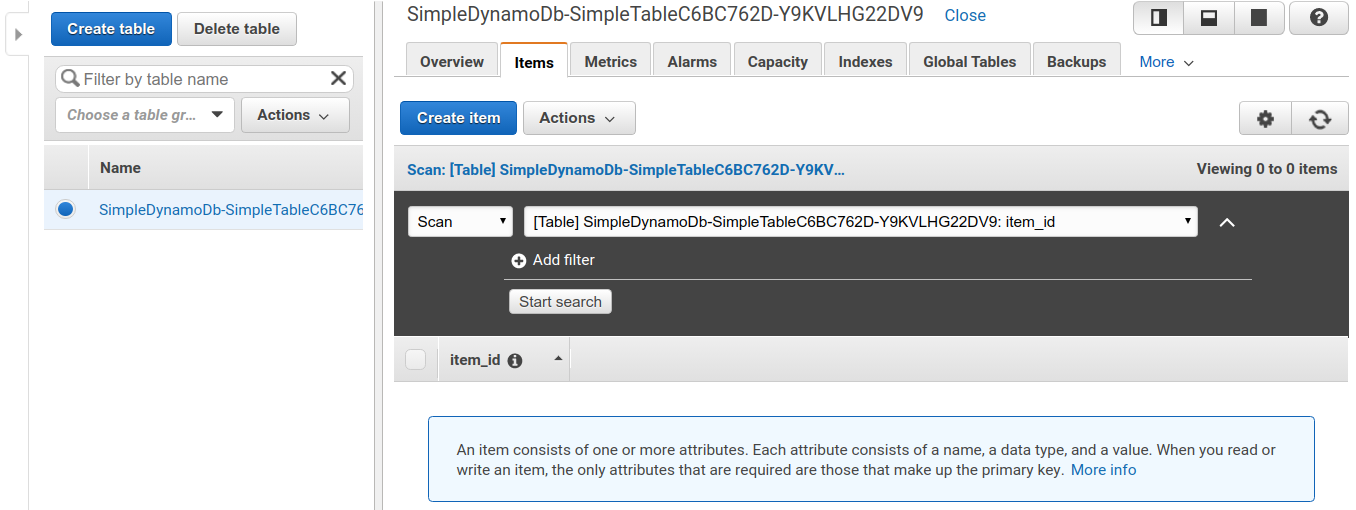
12.2.2. Read and write operations
Now, let’s practice read and write operations using the table that we just created. Here we will use Python and boto3 library.
First, we write a new record in the table. Open the file named simple_write.py in the hands-on directory. Inside the program, you will find the following code.
 1
 2
 3
 4
 5
 6
 7
 8
 9
10
11
12
13
14
import boto3
from uuid import uuid4
ddb = boto3.resource('dynamodb')

def write_item(table_name):
    table = ddb.Table(table_name)
    table.put_item(
    Item={
        'item_id': str(uuid4()),
        'first_name': 'John',
        'last_name': 'Doe',
        'age': 25,
        }
    )
If you read the code from the top, you will see that it first imports the boto3 library and then calls the dynamodb resource.
The write_item() function takes the name of the DynamoDB table as an argument.
Then, the put_item() method is called to write a new record to the DB.
The item has four attributes defined: item_id, first_name, last_name, and age.
The item_id corresponds to the partition key described above, and is given a random string using
UUID4
algorithm.
Now, let’s run simple_write.py.
Replace "XXXX" with the name of the table you deployed (a string starting with SimpleDynamoDb), and then execute the following command.
$ python simple_write.py XXXXLet’s check from the AWS console that the new record has been written correctly. Use the same procedure as Figure 89 to display the list of records in the table. You will find a new record as expected, as shown in Figure 90.
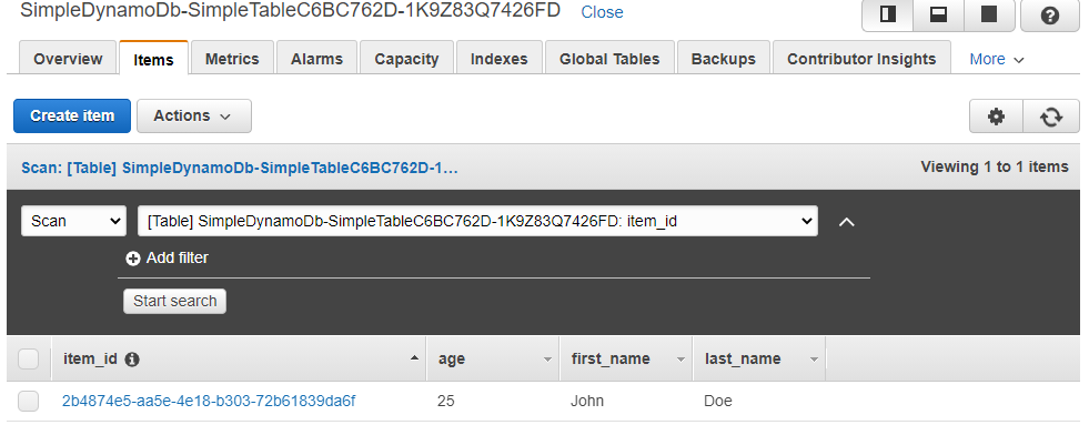
It is also possible to use boto3 to read elements from a table. Open the file named simple_read.py in the hands-on directory.
1
2
3
4
5
6
7
import boto3
ddb = boto3.resource('dynamodb')

def scan_table(table_name):
    table = ddb.Table(table_name)
    items = table.scan().get("Items")
    print(items)
By calling table.scan().get("Items"), all the records in the table are read out.
Let’s run this script with the following command (Don’t forget to replace the "XXXX" part correctly).
$ python simple_read.py XXXXYou should get an output showing the record we just added eariler.
12.2.3. Reading and writing a large number of records
The advantage of DynamoDB is that, as mentioned at the beginning, its processing capacity can be freely expanded according to the load.
To test the capability of DynamoDB, let’s simulate the situation where a large amount of data is written at once. In batch_rw.py, we have a short script to perform massive write operation to the database.
Run the following command (be sure to replace XXXX with the name of your table).
$ python batch_rw.py XXXX write 1000This command generates a thousand random data, and writes them to the database.
Furthermore, let’s search the database.
In the previous command, a random integer from 1 to 50 is assigned to the attribute age in each data.
To search and retrieve only those elements whose age is less than or equal to 2, you execute the following command.
$ python batch_rw.py XXXX search_under_age 2Let’s try running the above two commands several times to apply a simulated load to the database. You should see that the results are returned without any significant delay.
12.2.4. Deleting the stack
When you have had enough fun with DynamoDB, remember to delete the stack.
As in the previous hands-on sessions, you can delete the stack by executing the following command.
$ cdk destroy12.3. S3 hands-on
Coming soon…
13. Hands-on #6: Bashoutter
In the sixth and final hands-on session, we will create a simple web service using the serverless cloud technology we have learned so far. Specifically, let’s create a social networking service (SNS), named Bashoutter, where people can post their own haiku poems. (Haiku is a Japanese poetic form where it is consisted of 17 characters divided in to 5,5,7 character phrases.) By incorporating all the technologies such as Lambda, DynamoDB, and S3, a simple yet scalable social networking service that makes full use of serverless cloud will be born. By the end of this hands-on, we will deploy a modern-looking SNS shown in Figure 91.
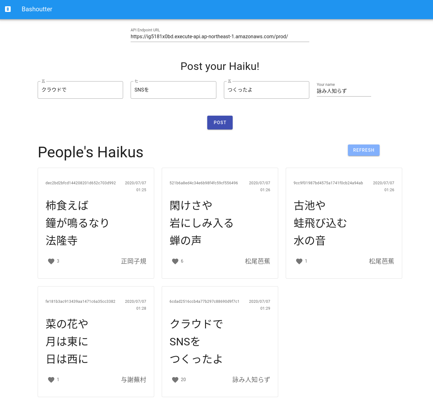
13.1. Preparation
The source code for the hands-on is available on GitHub at handson/bashoutter.
To run this hands-on, it is assumed that the preparations described in the first hands-on (Section 4.1) have been completed.
|
This hands-on exercise can be performed within the free AWS tier. |
13.2. Reading the application source code
13.2.1. API
In this application, we implement functions such as accepting haiku submissions from people, and retrieving a list of haiku from the database.
As a minimum design to realize this service, we will implement four REST APIs as shown in Table 11.
The APIs for basic data manipulation, such as posting, browsing, and deleting haiku, are provided.
In addition, PATCH /haiku/{item_id} is used to "like" the haiku specified by {item_id}.
|
Get a list of haiku |
|
Post a new haiku |
|
Like a haiku specified by |
|
Delete the haiku specified by |
|
The Open API Specification (OAS; formerly known as the Swagger Specification) is a description format for REST APIs. If the API specification is written according to the OAS, you can easily generate API documentation and client applications. API specification prepared for this project is also written according to the OAS. For more information, see official Swagger documentation. |
13.2.2. Application architecture
Figure 92 shows an overview of the application we are creating in this hands-on.
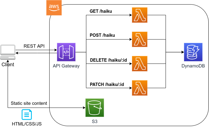
The summary of the system design is as follows:
-
API requests from the client are first sent to the API Gateway (described below), and then forwarded to the Lambda function specified by the API path.
-
An independent Lambda function is defined for each API path.
-
A database (powered by DynamoDB) is created to record the haiku information (author, text, submission date, etc.).
-
Give each Lambda function read and write access to DynamoDB.
-
Finally, we create an S3 bucket to deliver the static contents of the web page. Clients retrive HTML, CSS and JavaScript from this bucket and the contents will be displayed on a web browser.
Now, let us take a look at the main application code (handson/bashoutter/app.py).
  1
  2
  3
  4
  5
  6
  7
  8
  9
 10
 11
 12
 13
 14
 15
 16
 17
 18
 19
 20
 21
 22
 23
 24
 25
 26
 27
 28
 29
 30
 31
 32
 33
 34
 35
 36
 37
 38
 39
 40
 41
 42
 43
 44
 45
 46
 47
 48
 49
 50
 51
 52
 53
 54
 55
 56
 57
 58
 59
 60
 61
 62
 63
 64
 65
 66
 67
 68
 69
 70
 71
 72
 73
 74
 75
 76
 77
 78
 79
 80
 81
 82
 83
 84
 85
 86
 87
 88
 89
 90
 91
 92
 93
 94
 95
 96
 97
 98
 99
100
101
102
class Bashoutter(Stack):

    def __init__(self, scope: Construct, construct_id: str, **kwargs) -> None:
        super().__init__(scope, construct_id, **kwargs)

        (1)
        # dynamoDB table to store haiku
        table = ddb.Table(
            self, "Bashoutter-Table",
            partition_key=ddb.Attribute(
                name="item_id",
                type=ddb.AttributeType.STRING
            ),
            billing_mode=ddb.BillingMode.PAY_PER_REQUEST,
            removal_policy=cdk.RemovalPolicy.DESTROY
        )

        (2)
        bucket = s3.Bucket(
            self, "Bashoutter-Bucket",
            website_index_document="index.html",
            public_read_access=True,
            removal_policy=cdk.RemovalPolicy.DESTROY
        )
        s3_deploy.BucketDeployment(
            self, "BucketDeployment",
            destination_bucket=bucket,
            sources=[s3_deploy.Source.asset("./gui/dist")],
            retain_on_delete=False,
        )

        common_params = {
            "runtime": _lambda.Runtime.PYTHON_3_7,
            "environment": {
                "TABLE_NAME": table.table_name
            }
        }

        (3)
        # define Lambda functions
        get_haiku_lambda = _lambda.Function(
            self, "GetHaiku",
            code=_lambda.Code.from_asset("api"),
            handler="api.get_haiku",
            memory_size=512,
            **common_params,
        )
        post_haiku_lambda = _lambda.Function(
            self, "PostHaiku",
            code=_lambda.Code.from_asset("api"),
            handler="api.post_haiku",
            **common_params,
        )
        patch_haiku_lambda = _lambda.Function(
            self, "PatchHaiku",
            code=_lambda.Code.from_asset("api"),
            handler="api.patch_haiku",
            **common_params,
        )
        delete_haiku_lambda = _lambda.Function(
            self, "DeleteHaiku",
            code=_lambda.Code.from_asset("api"),
            handler="api.delete_haiku",
            **common_params,
        )

        (4)
        # grant permissions
        table.grant_read_data(get_haiku_lambda)
        table.grant_read_write_data(post_haiku_lambda)
        table.grant_read_write_data(patch_haiku_lambda)
        table.grant_read_write_data(delete_haiku_lambda)

        (5)
        # define API Gateway
        api = apigw.RestApi(
            self, "BashoutterApi",
            default_cors_preflight_options=apigw.CorsOptions(
                allow_origins=apigw.Cors.ALL_ORIGINS,
                allow_methods=apigw.Cors.ALL_METHODS,
            )
        )

        haiku = api.root.add_resource("haiku")
        haiku.add_method(
            "GET",
            apigw.LambdaIntegration(get_haiku_lambda)
        )
        haiku.add_method(
            "POST",
            apigw.LambdaIntegration(post_haiku_lambda)
        )

        haiku_item_id = haiku.add_resource("{item_id}")
        haiku_item_id.add_method(
            "PATCH",
            apigw.LambdaIntegration(patch_haiku_lambda)
        )
        haiku_item_id.add_method(
            "DELETE",
            apigw.LambdaIntegration(delete_haiku_lambda)
        )
| 1 | Here, a DynamoDB table is created to record the haiku information. |
| 2 | This part creates an S3 bucket to store and deliver the static site contents.
s3_deploy.BucketDeployment() configures the settings to automatically upload the necessary files when the stack is deployed. |
| 3 | This part defines the Lambda functions to be executed by each API path. The functions are written in Python 3.7 and the code can be found at handson/bashoutter/api/api.py. |
| 4 | The Lambda function defined in <3> is given read and write access to the database. |
| 5 | Here, the API Gateway is used to link each API path with the corresponding Lambda function. |
13.2.3. S3 bucket in Public access mode
Take a closer look at the part of the code where an S3 bucket is created.
1
2
3
4
5
6
bucket = s3.Bucket(
    self, "Bashoutter-Bucket",
    website_index_document="index.html",
    public_read_access=True,
    removal_policy=cdk.RemovalPolicy.DESTROY
)
What you should pay attention to here is the line public_read_access=True.
S3 has a feature called Public access mode.
When the public access mode is turned on, the files in the bucket can be viewed without authentication (i.e., by anyone on the Internet).
This setting is ideal for storing static content for public websites, and many serverless web services are designed this way.
When the public access mode is set, a unique URL such as http://XXXX.s3-website-ap-northeast-1.amazonaws.com/ is assigned to the bucket.
When a client accesses this URL, index.html in the bucket is returned to the client, and the page is loaded
(Note that we are specifying which file to be returned in the line website_index_document="index.html".)
|
When operating a web site for production, it is common to add the service called CloudFront to the S3 bucket in public access mode. CloudFront can be used to configure Content Delivery Nework (CDN) and encrypted HTTPS communication. For more information about CloudFront, please refer to official documentation "What is Amazon CloudFront?. In this hands-on session, CloudFront configuration was not performed to simplify the code, but readers who are interested may find the program at the following link helpful. |
|
The public S3 bucket is assigned a random URL by AWS.
If you want to host it in your own domain such as |
After creating an S3 bucket in public access mode, the following code is used to upload the website contents to the bucket upon deployment of the stack.
1
2
3
4
5
6
s3_deploy.BucketDeployment(
    self, "BucketDeployment",
    destination_bucket=bucket,
    sources=[s3_deploy.Source.asset("./gui/dist")],
    retain_on_delete=False,
)
With this code, the files in the directory ./gui/dist will be placed in the bucket when the deployment is started.
The directory ./gui/dist contains the static contents (HTML/CSS/JavaScript) of the website.
We will not explain the implementation details of the GUI here, but the code can be found at
handson/bashoutter/gui.
If you are interested, we recommend to read the source code.
13.2.4. API handler functions
When an API request comes, the function that performs the requested processing is called the handler function.
Let’s take a look at the part where the handler function for the GET /haiku API is defined in Lambda.
1
2
3
4
5
6
7
get_haiku_lambda = _lambda.Function(
    self, "GetHaiku",
    code=_lambda.Code.from_asset("api"),
    handler="api.get_haiku",
    memory_size=512,
    **common_params
)
Starting from the simplest part, memory_size=512 specifies the memory allocated for this function as 512MB.
code=_lambda.Code.from_asset("api") defines that the source code of the function should be retrieved from an external directory named api/.
Then, the line handler="api.get_haiku" specifies that get_haiku() function from api.py should be executed as a handler function.
Next, let’s look at the source code of get_haiku() function in api.py
(handson/bashoutter/api/api.py).
 1
 2
 3
 4
 5
 6
 7
 8
 9
10
11
12
13
14
15
16
17
18
19
20
ddb = boto3.resource("dynamodb")
table = ddb.Table(os.environ["TABLE_NAME"])

def get_haiku(event, context):
    """
    handler for GET /haiku
    """
    try:
        response = table.scan()

        status_code = 200
        resp = response.get("Items")
    except Exception as e:
        status_code = 500
        resp = {"description": f"Internal server error. {str(e)}"}
    return {
        "statusCode": status_code,
        "headers": HEADERS,
        "body": json.dumps(resp, cls=DecimalEncoder)
    }
In the line response = table.scan(), all the elements are retrieved from the DynamoDB table.
If no error occurs, the status code 200 is returned along with the haiku data, and if any error occurs, the status code 500 is returned.
By repeating the above operations for other APIs, handler functions for all APIs are defined.
|
In the handler function of |
13.2.5. Identity and Access Management (IAM)
Look at the following part of the code.
1
2
3
4
table.grant_read_data(get_haiku_lambda)
table.grant_read_write_data(post_haiku_lambda)
table.grant_read_write_data(patch_haiku_lambda)
table.grant_read_write_data(delete_haiku_lambda)
AWS has an important concept called IAM (Identity and Access Management). Although we have not mentioned it so far for the sake of simplicity, IAM is a very important concept in designing the cloud system on AWS. IAM basically defines what permissions a resource has over other resources. For example, in its default state, Lambda does not have any permissions to access other resources such as DynamoDB. Therefore, in order for a Lambda function to read or write DynamoDB data, an IAM must be granted to the Lambda function to allow such operation.
dynamodb.Table object in CDK has a convenient method grant_read_write_data(), which assigns IAM to other resources so that they can perform read and write operation to the database.
Similarly, the s3.Bucket object in CDK has a method grant_read_write() to allow reading and writing to the bucket.
Indeed, we used this method in Section 9 where we granted AWS Batch to write data to S3 bucket.
Interested readers can look back and check the code.
|
The best practice to manage IAM is that the minimam permissions necessary for the system to work should be assigned to each resource.
This will not only improve security of the system, but also reduce bugs by, for example, preventing unintended resources from reading or writing to the database.
For this reason, the above code grants only read permission to the handler of |
13.2.6. API Gateway
API Gateway is literally an gateway that forwards API requests to Lambda, EC2, and other resources according to the API request path ([fig:bashoutter_api_ gateway]). Then, the outputs of the processing performed by Lambda and EC2 are returned to the client via API Gateway. In cloud terminology, the server that stands between the client and the backend server whose job is to forward the connection according to the API path is called a router or a reverse proxy. Traditionally, routers are usually served by a dedicated virtual server. API Gateway, on the other hand, is a serverless router service where it achieves routing without a fixed server. API Gateway is dynamically launched only when the API request arrives. As a natural consequence of being serverless, it has the ability to automatically increase its routing capacity as the number of accesses increases.
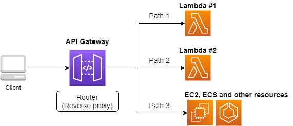
By deploying an API Gateway, one can easily build a system that can handle a large number of API requests (thousands to tens of thousands per second) without having to write codes. The summary of the API Gateway cost is shown in Table 12. API Gateway also offers free tier, so up to one million requests per month can be used for free.
| Number of Requests (per month) | Price (per million) |
|---|---|
First 333 million |
$4.25 |
Next 667 million |
$3.53 |
Next 19 billion |
$3.00 |
Over 20 billion |
$1.91 |
Let’s look at the source code.
 1
 2
 3
 4
 5
 6
 7
 8
 9
10
11
12
13
14
15
16
17
18
19
20
21
22
23
24
25
26
27
28
29
30
31
32
(1)
api = apigw.RestApi(
    self, "BashoutterApi",
    default_cors_preflight_options=apigw.CorsOptions(
        allow_origins=apigw.Cors.ALL_ORIGINS,
        allow_methods=apigw.Cors.ALL_METHODS,
    )
)

(2)
haiku = api.root.add_resource("haiku")
(3)
haiku.add_method(
    "GET",
    apigw.LambdaIntegration(get_haiku_lambda)
)
haiku.add_method(
    "POST",
    apigw.LambdaIntegration(post_haiku_lambda)
)

(4)
haiku_item_id = haiku.add_resource("{item_id}")
(5)
haiku_item_id.add_method(
    "PATCH",
    apigw.LambdaIntegration(patch_haiku_lambda)
)
haiku_item_id.add_method(
    "DELETE",
    apigw.LambdaIntegration(delete_haiku_lambda)
)
| 1 | First, an empty API Gateway is created by api = apigw.RestApi(). |
| 2 | Next, we add add the API path /haiku by calling the method api.root.add_resource(). |
| 3 | Next, add_method() is called to define the GET and POST methods for the /haiku path. |
| 4 | Similarly, haiku.add_resource("{item_id}") adds the API path /haiku/{item_id}. |
| 5 | Finally, add_method() is used to define PATCH and DELETE methods in the path /haiku/{item_id}. |
As you can see, API Gateway is very simple to use. All you need to do is to sequentially describe the API path and the methods that will be executed.
|
When you create a new API with this program, a random URL will be assigned as the API endpoint.
If you want to host it in your own domain such as |
|
When we created a new API with API Gateway, the parameter |
13.3. Deploying the application
The deployment procedure is almost the same as the previous hands-on.
Here, only the commands are listed (lines starting with # are comments).
If you have forgotten the meaning of each command, review the first hands-on.
You should not forget to set the access key (Section 14.3).
# move to the project directory
$ cd intro-aws/handson/bashoutter

# create venv and install dependent libraries
$ python3 -m venv .env
$ source .env/bin/activate
$ pip install -r requirements.txt

# Deploy!
$ cdk deploy
If the deployment is successful, you should see an output like Figure 94.
In the output you should find Bashoutter.BashoutterApiEndpoint = XXXX and Bashoutter.BucketUrl = YYYY.
We will use these string values later, so be sure to make notes of them.
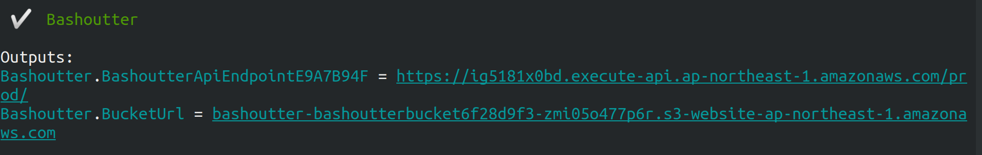
cdk deployNow, let’s log in to the AWS console and check the deployed stack. First, go to the API Gateway page. You will see a screen like Figure 95, where you can check the list of deployed API endpoints.
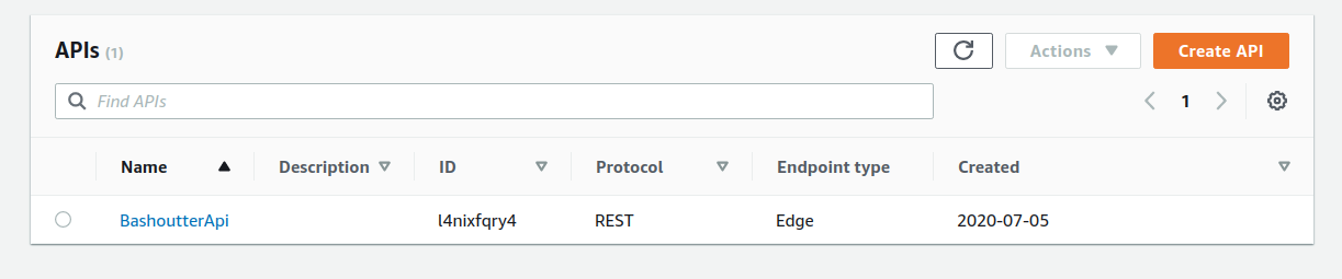
By clicking on the API named "BashoutterApi", you can move to a screen like Figure 96 and view detailed information.
You can see that GET /haiku, POST /haiku, and other APIs are defined.
Click on each method to see detailed information about that method. In addition to the aforementioned routing functions, API Gateway can also be used to add authentication. We won’t be using these authentication feature in this hands-on, but this feature will be useful in many web applications. Next, in Figure 96, notice that the Lambda functions called by this API is shown in the area circled in red. Clicking on the function name will take you to the console of the corresponding Lambda function, where you can view the contents of the function.
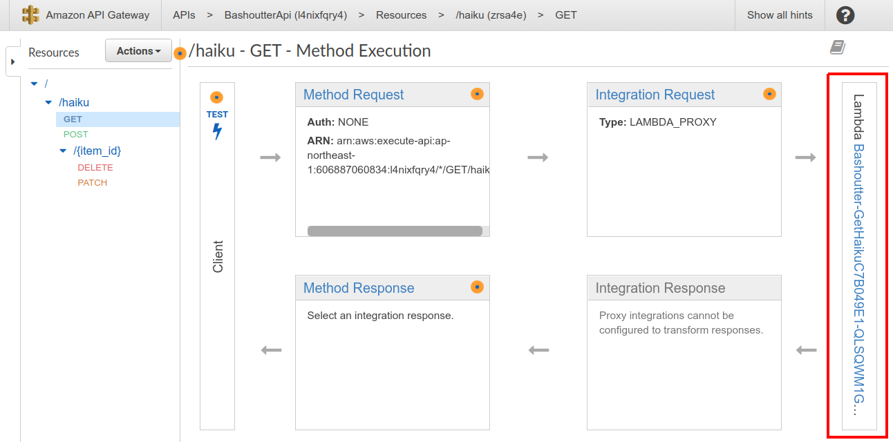
Next, we will move to the S3 console.
There, you should be able to find a bucket whose name starts with bashouter-XXXX (where XXXX is some random string) (Figure 97).
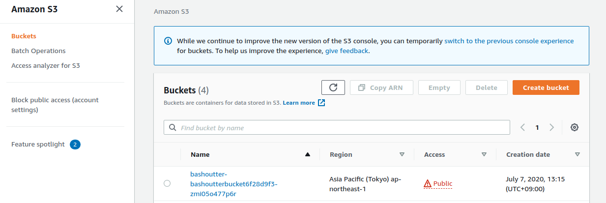
Let’s check the contents of the bucket by clicking on the bucket name.
You will find the main html document, index.html, along with css/, js/ and other directories which store the components to render the web page (Figure 98).
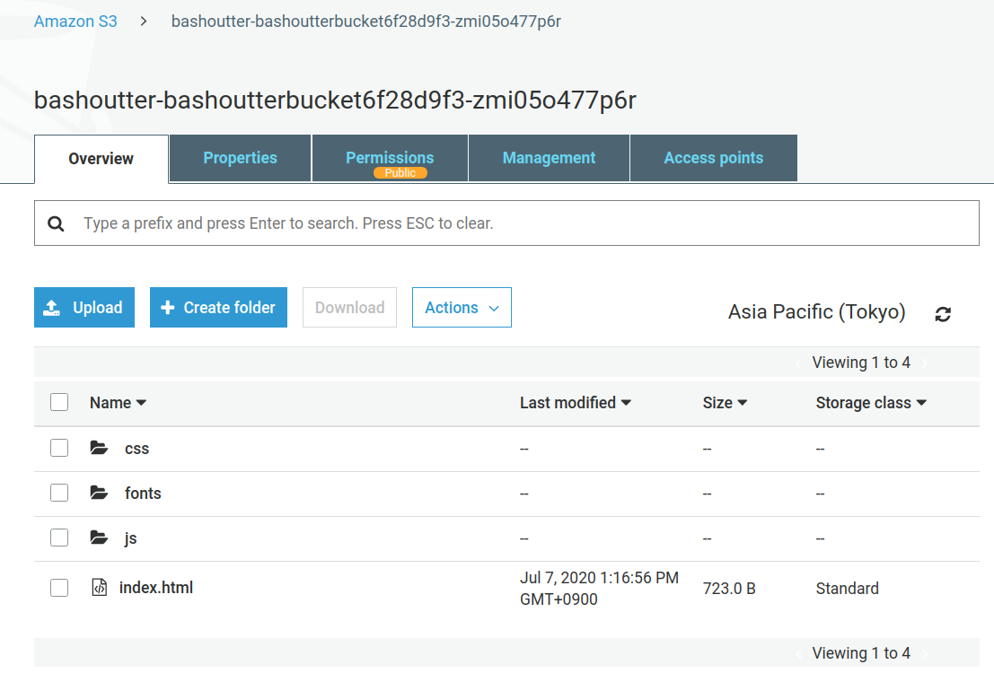
13.4. Sending API requests
Now, let’s actually send API requests to the deployed application. First, let’s practice sending API requests from the command line.
Here we use a simple HTTP client tool,
HTTPie,
to send HTTP API requests from the command line.
HTTPie is installed together with the Python virtual environment (venv) when we deployed the stack.
To make sure that the installation is successful, activate the virtual environment and type http on the command line.
If you get a help message, you are ready to go.
First, set the URL of the API endpoint to a command line variable (the XXXX string from Bashoutter.BashoutterApiEndpoint = XXXX).
$ export ENDPOINT_URL=XXXXThen, obtain a list of haiku by sending GET /haiku API.
$ http GET "${ENDPOINT_URL}/haiku"Unfortunately, there is no haiku registered in the database at this moment, so you will see an empty array ([]) as return.
Next, let’s post our very first haiku using POST /haiku.
$ http POST "${ENDPOINT_URL}/haiku" \
username="Mastuo Bashou" \
first="the stillness" \
second="penetrating the rock" \
third="a cicada's cry"
The following output will be obtained.
HTTP/1.1 201 Created
Connection: keep-alive
Content-Length: 49
Content-Type: application/json
....
{
    "description": "Successfully added a new haiku"
}
It seems we successfully submited a new haiku. Let’s confirm that the haiku is indeed added to the database by calling the GET request again.
$ http GET "${ENDPOINT_URL}/haiku"

HTTP/1.1 200 OK
Connection: keep-alive
Content-Length: 258
Content-Type: application/json
...
[
    {
        "created_at": "2020-07-06T02:46:04+00:00",
        "first": "the stillness",
        "item_id": "7e91c5e4d7ad47909e0ac14c8bbab05b",
        "likes": 0.0,
        "second": "penetrating the rock",
        "third": "a cicada's cry",
        "username": "Mastuo Bashou"
    }
]
Excellent!
Next, let’s add a "like" to this haiku by calling PATCH /haiku/{item_id}.
To do this, run the following command after replacing XXXX with the ID of the haiku that you created in the previous command (i.e. item_id in the response text).
$ http PATCH "${ENDPOINT_URL}/haiku/XXXX"You should get the output {"description": "OK"}.
We confirm that the number of likes has increased by 1 by sending the GET request one more time.
$ http GET "${ENDPOINT_URL}/haiku"
...
[
    {
        ...
        "likes": 1.0,
        ...
    }
]
Lastly, we delete the haiku by sending the DELETE request.
Run the following command after replacing XXXX with the ID of the haiku.
$ http DELETE "${ENDPOINT_URL}/haiku/XXXX"If we send GET request, the return will be an empty array ([]).
Now we were able to validate that the basic APIs for posting, retrieving, deleting, and adding "likes" to haiku are working properly.
13.5. Simulating a large simultaneous API request
In the previous section, we manually posted haiku one by one. In a social networking service with a large number of users, several thousand haiku would be posted every second. By adopting a serverless architecture, we have built a system that can easily handle such instantaneous heavy access. To demonstrate this point, let’s simulate a situation where a large number of APIs are sent to the system.
In
handson/bashoutter/client.py,
we provide a short script to send many API requests simultaneously.
By using this script, we can send POST /haiku API request for a specified number of times.
As a test, we will send the API request for 300 times. Run the following command.
$ python client.py $ENDPOINT_URL post_many 300The execution would be completed in a matter of seconds. If this API had been supported by a single server, it would have taken much longer to process such a large number of requests. In the worst case, it might have even led to a server shutdown. The serverless application we have created is a very simple yet scalable cloud system that can handle hundreds of requests every second. Did you get a glimpse of the benefits and power of a serverless cloud?
|
If you submit a large number of haiku using the above command, the database will be filled with useless data. To completely empty the database, use the following command. |
13.6. Interacting with Bashoutter GUI
In the previous part, we practiced sending APIs from the command line. In a web application, the exact same thing is done behind a web browser to display the contents of a page (see Figure 74). Lastly, let’s see what happens when the API is integrated with the GUI.
Let’s check the URL given by Bashoutter.BucketUrl= that is output on the command line when we deployed the stack (Figure 94).
As mentioned earlier, this is the URL of the S3 bucket in public access mode.
Open a web browser and enter the URL of S3 in the address bar to access it. You should see a page like shown in Figure 99.
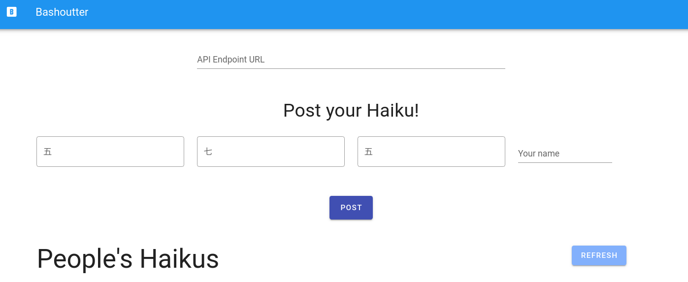
When the page is loaded, enter the URL of the API Gateway you deployed in the text box at the top that says "API Endpoint URL". (In this application, the API Gateway URL is randomly assigned, so the GUI is designed like this.) Then, press the "REFRESH" button on the screen. If you have already registered some haiku in the database, you will see a list of haiku. Click on the heart icon at the bottom left of each haiku to give it a "like" vote.
To submit a new haiku, enter the new phrase and the name of the author, then press "POST". After pressing "POST", be sure to press the "REFRESH" button again to retrieve the latest list of haiku from the database.
13.7. Deleting the stack
This concludes the Bashoutter project! We created an SNS that can be accessed from anywhere in the world via the Internet. As we demonstrated in [simulating_many_apis], Bashoutter can scale flexibly to handle a large number of simultaneous access without delay. Although it is extremely simple, it satisfies the basic requirements for an modern and scalable web service!
When you have enjoyed Bashoutter application, don’t forget to delete the stack.
To delete the stack from the command line, use the following command.
$ cdk destroy|
Depending on the version of CDK, To do this from the AWS console, go to the S3 console, open the bucket, select all the files, and execute "Actions" → "Delete". To do this from the command line, use the following command. Remember to replace <BUCKET NAME> with the name of your bucket. |
13.8. Short summary
This is the end of Part III of this book.
In Part III, we focused on how to create web applications and databases that can be used by the general public as an application of cloud computing. Along the way, we explained the traditional design of cloud systems and the latest design method called serverless architecture. In Section 12, we practiced serverless architecture in AWS by using Lambda, S3, and DynamoDB. Finally, in Section 13, we integrated these serverless technologies to create a simple web application called "Bashoutter".
Through these exercises, we hope you have gained a better understanding of how web services are developed and maintained in the real world. We also hope that this hands-on session was a good starting point for you to create amazing web application yourself.
14. Appendix: Environment setup
To read through this book, you need to set up an environment on your local machine to run the hands-on programs. Assuming that you are a beginner in AWS and the command line, this chapter will briefly explain how to install the necessary software and libraries. A brief table of contents is shown below. If you have already built your environment, you need to read through only the relevant parts.
-
Creating an AWS account (Section 14.1)
-
Creating AWS access key (Section 14.2)
-
Installing AWS CLI (Section 14.3)
-
Installing AWS CDK (Section 14.4)
-
Installing WSL (Section 14.5)
-
Installing Docker (Section 14.6)
-
Quick tutorial on Python venv (Section 14.7)
-
Working with Docker image for the hands-on exercises (Section 14.8)
The OS can be Linux, Mac, or Windows. Windows users are assumed to use Windows Subsytem for Linux (WSL) (Section 14.5).
You can also use the Docker image to run the hands-on programs in this book. This will be useful for readers who know how to use Docker, as it allows them to skip AWS CLI/CDK and Python installation.
14.1. Creating an AWS account
In order to try the hands-on exercises provided in this book, you need to create your own AWS account. Detailed instructions for creating an account can be found at official documentation, so please refer to that as well. Follow the steps below to create an account.
First, access AWS Management Console from your web browser, and click Create an AWS Account in the upper right corner.
(Figure 100, boxed with a solid line).
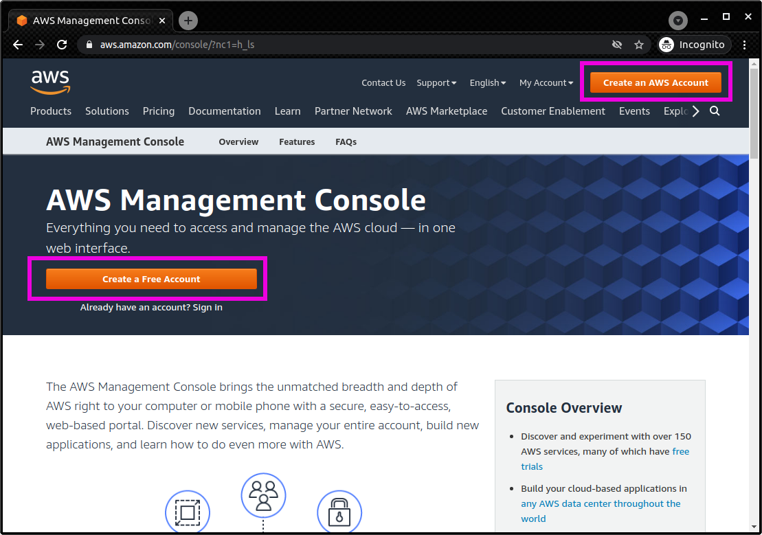
Then, you will be taken to a page where you register your email address and password (Figure 101).
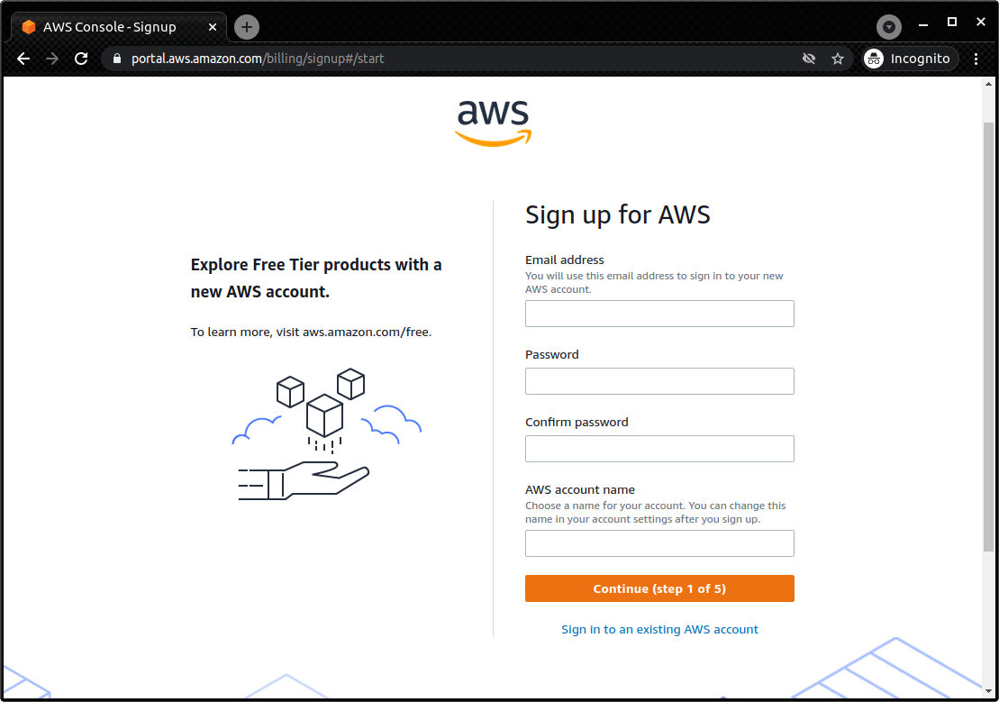
Next, you will be asked to enter your address, phone number, and other information (Figure 102).
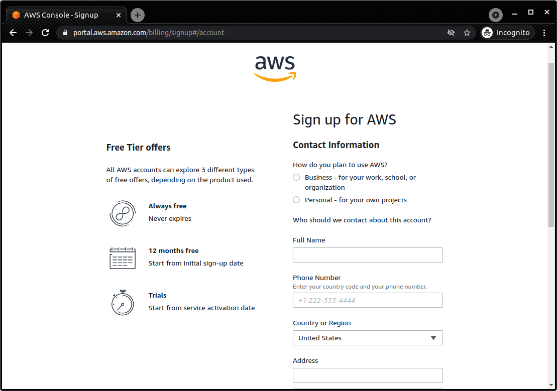
Next, you will be asked to register your credit card information (Figure 103). If you are using AWS as an individual, you will be billed for your usage via your credit card. Note that you cannot start using AWS without registering your credit card information.
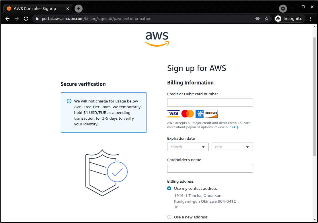
On the next page, you will be asked to verify your identity using SMS or voice message on your cell phone (Figure 104). Select your preferred authentication method and enter your cell phone number.
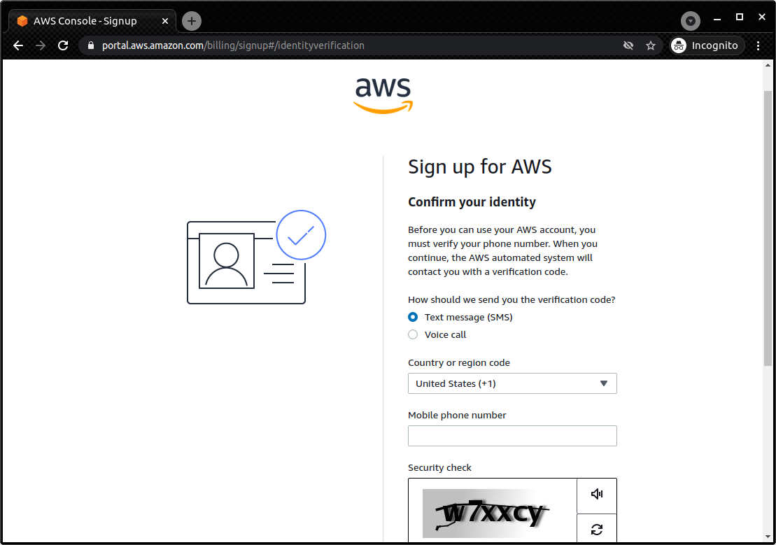
After successfully verifying your identity, you will be asked to select a support plan (Figure 105). You can just select the Basic support plan, which is free.
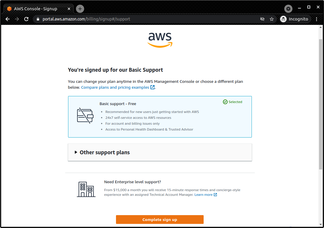
These steps will complete the creation of your account (Figure 106). Let’s log in and see if we can access the AWS console.
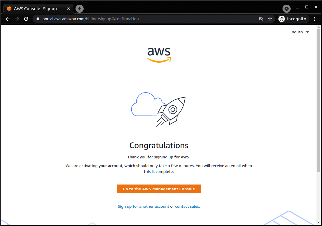
14.2. Creating AWS access key
AWS access key is a key used for user authentication when operating the AWS API from the AWS CLI or AWS CDK. To use the AWS CLI/CDK, you need to issue a secret key first. For more information on AWS secret keys, please refer to the official documentation "Understanding and getting your AWS credentials".
-
First, log in to your AWS console
-
Then, click on your account name in the upper right corner of the screen, and select "My Security Credentials" from the pull-down menu (Figure 107)
-
Under "Access keys for CLI, SDK, & API access", find the button that says "Create accesss key" and click it (Figure 108)
-
Record the displayed access key ID and secret access key (if you close the window, they will not be displayed again)
-
If you forget your key, you can reissue it by the same procedure
-
Use the issued secret key by writing it to the file
~/.aws/credentialsor by setting it to an environment variable (also see Section 14.3)
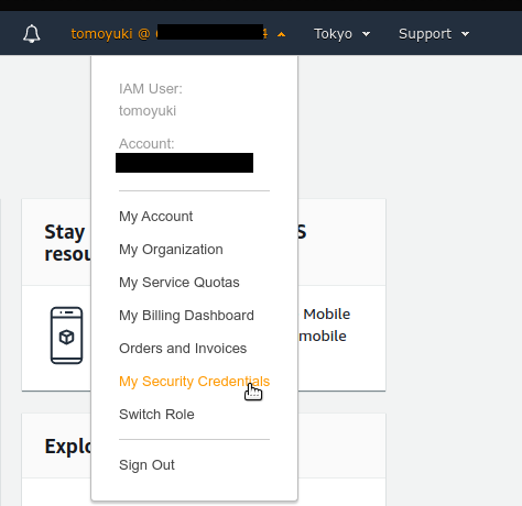
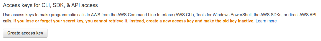
14.3. Installing AWS CLI
This is a brief description of the installation procedure for Linux at the time of writing. Please remember to always check official documentation for the latest information, as it may change in future versions.
Installation of AWS CLI version 2 can be done by downloading and executing the installation script:
$ curl "https://awscli.amazonaws.com/awscli-exe-linux-x86_64.zip" -o "awscliv2.zip"
$ unzip awscliv2.zip
$ sudo ./aws/install
To confirm that the installation is successful, type the following command to see if the version information is displayed.
$ aws --versionOnce the installation is complete, run the following command to finish the initial set up (also see official documentation "Configuring the AWS CLI").
$ aws configureWhen you execute this command, you will be prompted to enter the AWS Access Key ID and AWS Secret Access Key.
See Section 14.2 for issuing access keys.
The command also asks for the Default region name.
You can specify your favorite region (e.g. ap-northeast-1 = Tokyo) here.
The last entry, Default output format, should be json.
After completing this command, you should see files named ~/.aws/credentials and ~/.aws/config, where the relevant information is stored.
To be sure, you can use the cat command to check the contents.
$ cat ~/.aws/credentials
[default]
aws_access_key_id = XXXXXXXXXXXXXXXXXX
aws_secret_access_key = YYYYYYYYYYYYYYYYYYY

$ cat ~/.aws/config
[profile default]
region = ap-northeast-1
output = json
Authentication key information is stored in ~/.aws/credentials, and AWS CLI settings are stored in ~/.aws/config.
By default, a profile is saved with the name [default].
If you want to use several different profiles, follow the default example and add a profile with your favorite name.
In order to swtich your profile when executing AWS CLI commands, add --profile parameter:
$ aws s3 ls --profile myprofileIf you find that adding --profile each time you run a command is tedious, you can set the environemntal variable named AWS_PROFILE.
$ export AWS_PROFILE=myprofileOr, you can set the access key information in the environmental variables.
export AWS_ACCESS_KEY_ID=XXXXXX
export AWS_SECRET_ACCESS_KEY=YYYYYY
export AWS_DEFAULT_REGION=ap-northeast-1
These environmental variables have higher priority than the profiles defined in ~/.aws/credentials, so the profie defined by environemtal variables are used (see also
official documentation "Configuring the AWS CLI").
14.4. Installing AWS CDK
This is a brief description of the installation procedure for Linux at the time of writing. Please remember to always check official documentation for the latest information, as it may change in future versions.
If you have Node.js installed, you can install AWS CDK by the following command:
$ sudo npm install -g aws-cdk|
The hands-on exercises were developed with AWS CDK version 1.100. Since CDK is a library under active development, the API may change in the future. If errors occur due to API changes, it is recommended to use version 1.100.0. |
To confirm that the installation is successful, type the following command to see if the version information is displayed.
$ cdk --versionOnce the installation is complete, run the following command to finish the initial set up:
$ cdk bootstrap|
When you run |
|
The configuration of AWS credentials for CDK is basically the same as that of AWS CLI. See Section 14.3 for details. |
14.5. Installing WSL
In this book, the commands are basically written with a UNIX terminal in mind. Linux and Mac users can use the terminal that comes standard with their OS. If you are using Windows, we recommend that you use Windows Subsystem for Linux (WSL) to create a virtual Linux environment. Other tools that emulate the Linux environment, such as Cygwin, are also acceptable, but the programs in this book have been tested only on WSL.
WSL is software officially provided by Microsoft to run a Linux virtual environment on a Windows OS. You can select the Linux distribution you want, such as Ubuntu, and use basically all programs and software made for Linux.
At the time of writing, WSL 2 is the latest release. In the following, we will explain the steps to install WSL 2. For more details, also refer to the official documentation.
As a prerequisite, the OS must be Windows 10 (Pro or Home edition). Furthermore, make sure that the version of Windows 10 you are using supports WSL. For X64 systems, it must be Version 1903, Build 18362 or higher. If the version does not support WSL, update Windows first.
First, start PowerShell with administrator privileges (Figure 109).
To do this, type powershell in the search bar of the Windows menu in the lower left corner, and you should find the PowerShell program.
Then, right-click on it, and select Run as administrator to launch.
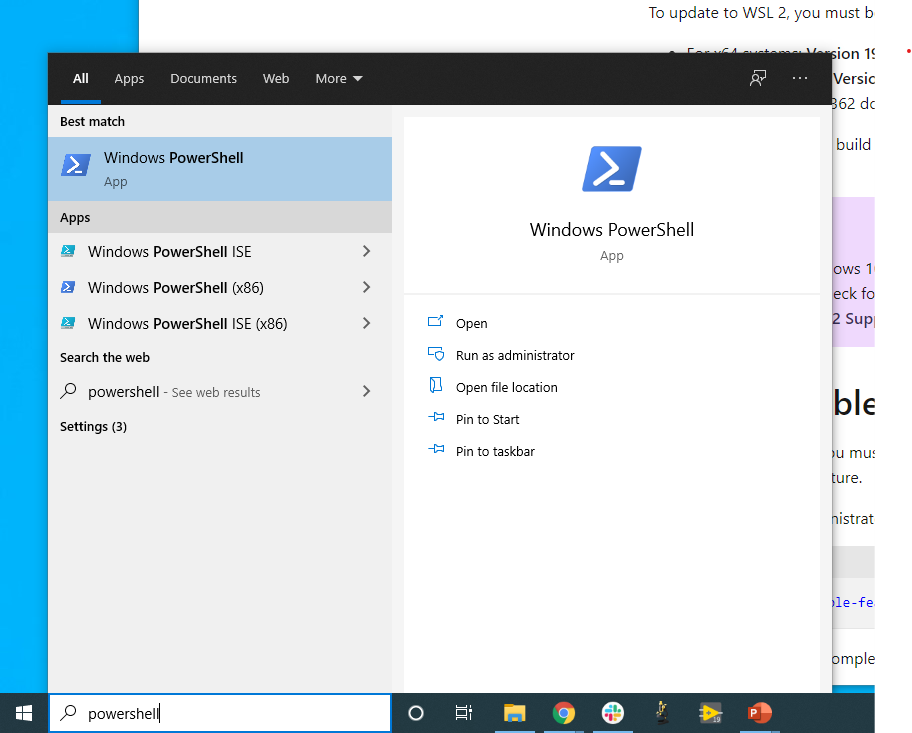
Once the PowerShell is ready, execute the following command:
dism.exe /online /enable-feature /featurename:Microsoft-Windows-Subsystem-Linux /all /norestartAfter the execution, make sure that the command outputs the line “The operation completed successfully”.
Now WSL is enabled on your Windows.
Next, using the same PowerShell started with administrator privileges, execute the following command:
dism.exe /online /enable-feature /featurename:VirtualMachinePlatform /all /norestartAfter the execution, make sure that the command outputs the line “The operation completed successfully”.
Once this is done, restart your computer.
Next, download Linux kernel update package from the following link: https://wslstorestorage.blob.core.windows.net/wslblob/wsl_update_x64.msi
Double-click on the downloaded file to run it. Follow the dialog to complete the installation.
After that, come back to PowerShell and run the following command:
wsl --set-default-version 2Lastly, install the Linux distribution of your choice. In this tutorial, let’s install Ubuntu 20.04.
Launch the Microsoft Store app and type Ubuntu in the search bar.
Open Ubuntu 20.04 LTS and click the "Get" button (Figure 110).
Wait for a while, and the installation of Ubuntu 20.04 will be completed.
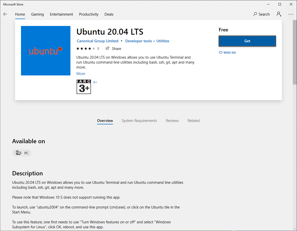
The first time you start Ubuntu 20.04, the initial setup will start automatically and you will have to wait for a few minutes. After the initial setup, you will be prompted to enter your user name and password.
This completes the installation of WSL2.
Let’s launch WSL2!
Type Ubuntu in the search bar of the Windows menu in the lower left corner, and you should find Ubuntu 20.04 (Figure 111).
Click on it to start it.
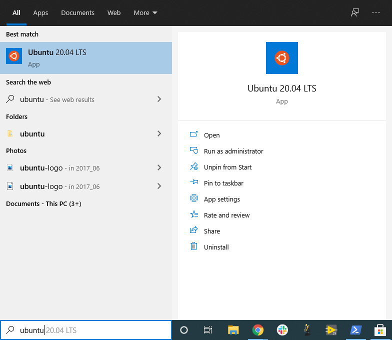
This should bring up a black terminal screen (Figure 112).
Try typing ls, top, etc. to confirm that WSL is working properly.
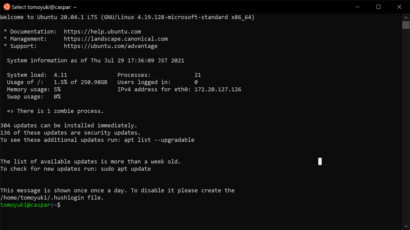
Optionally, you can install Windows Terminal. Windows Terminal is a tool provided by Microsoft, which gives you more functional and comfortable interface to work with WSL. We recommend that you to install this tool.
14.6. Installing Docker
The installation method of Docker varies depending on the OS.
Mac users should install Docker Desktop.
All you need do is to download Docker Desktop for Mac from
Docker’s website,
double-click the downloaded file, and then drag it to the Applications folder.
For more information, see
official documentation.
Windows users should install Docker Desktop.
WSL 2 must be installed in your machine prior to installing Docker Desktop.
See
official documentation
for more information.
After installing Docker Desktop, you can use the docker command from WSL.
For Linux users (especially Ubuntu users), there are several approaches to installation. For more information, please refer to official documentation. The simplest approach is to use the official Docker installation script. In this case, the following command will install Docker.
$ curl -fsSL https://get.docker.com -o get-docker.sh
$ sudo sh get-docker.sh
In the default installation, only the root user is allowed to use the docker command.
Therefore, you need to add sudo to the command every time.
If you find this cumbersome, follow these steps to add the user you are working with to the docker group
(For more information see
official documentation "Post-installation steps for Linux").
The first step is to add a group named docker.
Depending on your installation, the docker group may already be created.
$ sudo groupadd dockerNext, add the user you are currently using to the docker group.
$ sudo usermod -aG docker $USEROnce this is done, log out and log back in. The changes to the group will be reflected in your terminal session.
To check if the settings are correct, run the following command.
$ docker run hello-worldIf you can run the container withoug adding sudo, the setting is complete.
14.7. Quick tutorial on Python venv
Many of you may have experienced a situation where a program given to you by someone else does not work because of the library version mismatch. If you have only one Python environment in your machine, you will have to re-install the correct version every time you switch projects. This is a lot of work!
To make code sharing smoother, library versions should be managed on a project-by-project basis. This is made possible by tools called Python virtual environments. Programs such as venv, pyenv, and conda are often used for this purpose.
Among them, venv is very useful because it is included in Python as a standard feature.
Tools like pyenv and conda require separate installation, but they have their own advantages.
To create a new virtual environment using venv, you run the following command.
$ python -m venv .envThis command will create a directory .env/ in which the libraries for this virtual environment will be saved.
To activate this new virtual environment, you run the following command.
$ source .env/bin/activateNotice that the shell prompt starts with (.env) (Figure 113).
This is a sign that signifies, "You are now in a venv".
When the virtual Python environment is activated, all subsequent pip commands will install libraries under .env/ directory.
In this way, you can separate the version of the library used for each project.
In Python, it is common practice to describe the dependent libraries in a file called requirements.txt.
If a project you are workin on has a requirements.txt file defined, you can use the following command to install dependent libraries and reproduce the Python environment.
$ pip install -r requirements.txt|
You can give arbitrary name to the directory where the virtual environment is saved by |
14.8. Working with Docker image for the hands-on exercise
We prepared a Docker image with Node.js, Python, AWS CDK, etc. installed, which is necessary to run the hands-on exercises. Using this image, you can run the hands-on code immediately without having to install anything on your local machine.
|
Some of the commands in the hands-on must be executed outside of Docker (i.e. in the real environment on your local machine). These are described as notes in the corresponding part of the hands-on. |
Docker image is provided at the author’s Docker Hub repository. The build file for the Docker image is available at GitHub.
Use the following command to launch the container.
$ docker run -it tomomano/labc:latestThe first time you run the command, the image will be downloaded (pulled) from Docker Hub. From the second time onward, the locally downloaded image will be used.
When the container is started, you should see an interactive shell like the following (note the -it option at startup).
root@aws-handson:~$In the container shell, if you type the ls command, you should find a directory handson/.
Now you move to this directory.
$ cd handson
You will find a directory for each hands-on. Then, you can move the directory for each exercise, create a Python virtual environment, and deploy the stack (see Section 4.4, etc.). Since each hands-on uses different dependent libraries, the design is to create a virtualenv for each hands-on.
Don’t forget to set your AWS credentials.
An easy way to do this is to set environment variables such as AWS_ACCESS_KEY_ID as described in Section 14.3.
Alternatively, if your credentials are stored in local machine’s ~/.aws/credentials, you can mount this directory in the container and refer to the same credentials file from inside the container.
If you take this option, start the container with the following command.
$ docker run -it -v ~/.aws:/root/.aws:ro tomomano/labc:latestThis allows you to mount ~/.aws on the local machine to /root/.aws in the container.
The :ro at the end means read-only.
It is recommended to add the read-only flag to prevent accidental rewriting of important authentication files.
|
|